Download to read offline


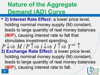
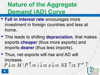
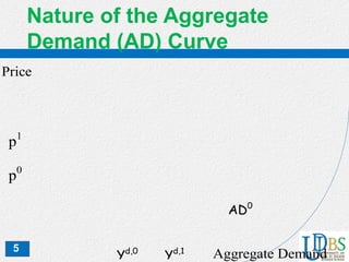
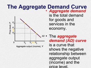
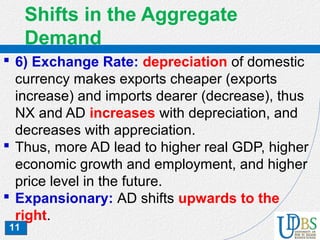
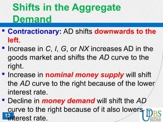
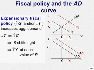
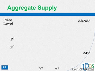
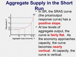
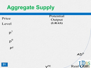
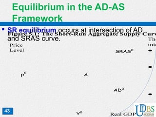
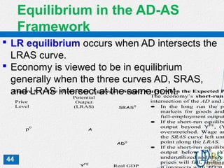
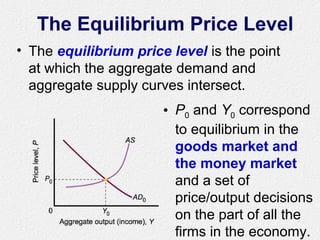
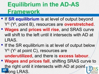


This document is a lecture on macroeconomics from the University of Dar Es Salaam Business School. It discusses the aggregate demand curve and how it slopes downward as the price level decreases due to wealth, interest rate, and exchange rate effects. It also discusses the short-run aggregate supply curve and how it slopes upward in the short-run as higher prices lead to increased output. Factors that can shift the aggregate demand and supply curves, such as fiscal policy, monetary policy, and cost shocks are also examined.