Downloaded 109 times


![Contd….
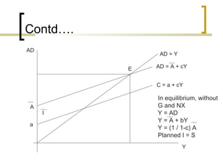
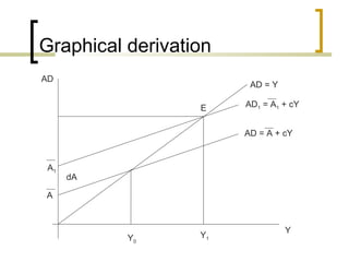
In equilibrium, Y = AD
Y = A + c(1-t) Y
Y [1-c(1-t)] = A where A = a+ cTR+ I+ G
Y = A / 1-c(1-t)
Multiplier in presence of taxes = α = 1 / 1–c(1-t)
Government spending can increase A by the
amount of purchases G and by the amount of
induced spending out of transfers bTR
Increased A will increase Y depending on the value
of MPC and tax rate
When tax rates (t) are higher, value of multiplier is
lower](https://image.slidesharecdn.com/aggregatedemandandsupply-130323071201-phpapp01/85/Aggregate-demand-and-supply-15-320.jpg)


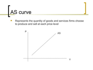
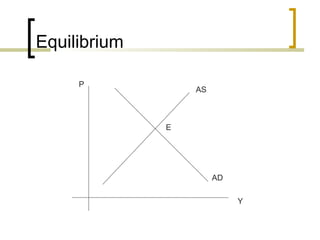

This document discusses key concepts in Keynesian economics including aggregate demand, aggregate supply, and their relationship. It explains that according to Keynesian theory, output and employment are determined by aggregate demand. The aggregate demand curve slopes positively, showing the total quantity demanded at each price level in the economy. The aggregate supply curve can be upward-sloping in the short-run due to sticky wages and prices. The intersection of the aggregate demand and supply curves indicates the general equilibrium in the economy.