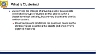
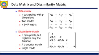
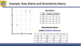
The document provides an overview of clustering and cluster analysis, focusing on the measurement of similarity and dissimilarity among data objects using various distance measures. It discusses clustering techniques and their applications across different fields, and highlights important concepts such as intra-class similarity, inter-class dissimilarity, and methods like k-means and hierarchical clustering. Additionally, it covers criteria for evaluating clustering quality and different approaches to clustering, including partitioning, density-based, and model-based methods.

1. Sanjivani Rural Education Society’s
Sanjivani College of Engineering, Kopargaon-423 603
(An Autonomous Institute, Affiliated to Savitribai Phule Pune University, Pune)
NACC ‘A’ Grade Accredited, ISO 9001:2015 Certified
Department of Computer Engineering
(NBA Accredited)
Prof. S. A. Shivarkar
Assistant Professor
Contact No.8275032712
Email- shivarkarsandipcomp@sanjivani.org.in
Subject- Data Mining and Warehousing (CO314)
Unit –IV: Cluster Analysis: Measuring Similarity &
Dissimilarity

2. Content
 Measuring Data Similarity and Dissimilarity, Proximity Measures for Nominal
Attributes and Binary Attributes, interval scaled;
 Dissimilarity of Numeric Data: Minskowski Distance Euclidean distance and
Manhattan distance
 Proximity Measures for Categorical, Ordinal Attributes, Ratio scaled
variables;
 Dissimilarity for Attributes of Mixed Types, Cosine Similarity,
 Partitioning methods- k-means, kmedoids, outlier detection.

3. What is Clustering?
 Clustering is the process of grouping a set of data objects
into multiple groups or clusters so that objects within a
cluster have high similarity, but are very dissimilar to objects
in other clusters.
 Dissimilarities and similarities are assessed based on the
attribute values describing the objects and often involve
distance measures

4. What is Cluster Analysis?
 Cluster: A collection of data objects
 similar (or related) to one another within the same group
 dissimilar (or unrelated) to the objects in other groups
 Cluster analysis (or clustering, data segmentation, …)
 Finding similarities between data according to the
characteristics found in the data and grouping similar
data objects into clusters
 Unsupervised learning: no predefined classes (i.e., learning
by observations vs. learning by examples: supervised)
 Typical applications
 As a stand-alone tool to get insight into data distribution
 As a preprocessing step for other algorithms

5. Clustering for Data Understanding and Applications
 Biology: taxonomy of living things: kingdom, phylum, class, order, family,
genus and species
 Information retrieval: document clustering
 Land use: Identification of areas of similar land use in an earth observation
database
 Marketing: Help marketers discover distinct groups in their customer bases,
and then use this knowledge to develop targeted marketing programs
 City-planning: Identifying groups of houses according to their house type,
value, and geographical location
 Earth-quake studies: Observed earth quake epicenters should be clustered
along continent faults
 Climate: understanding earth climate, find patterns of atmospheric and ocean
 Economic Science: market research

6. Quality: What Is Good Clustering?
 A good clustering method will produce high quality
clusters
 high intra-class similarity: cohesive within clusters
 low inter-class similarity: distinctive between clusters
 The quality of a clustering method depends on
 the similarity measure used by the method
 its implementation, and
 Its ability to discover some or all of the hidden patterns

7. Measure the Quality of Clustering
 Dissimilarity/Similarity metric
 Similarity is expressed in terms of a distance function, typically metric:
d(i, j)
 The definitions of distance functions are usually rather different for
interval-scaled, boolean, categorical, ordinal ratio, and vector variables
 Weights should be associated with different variables based on
applications and data semantics
 Quality of clustering:
 There is usually a separate “quality” function that measures the
“goodness” of a cluster.
 It is hard to define “similar enough” or “good enough”
 The answer is typically highly subjective

8. Similarity and Dissimilarity
 Similarity
 Numerical measure of how alike two data objects are
 Value is higher when objects are more alike
 Often falls in the range [0,1]
 Dissimilarity (e.g., distance)
 Numerical measure of how different two data objects
are
 Lower when objects are more alike
 Minimum dissimilarity is often 0
 Upper limit varies
 Proximity refers to a similarity or dissimilarity

9. Data Matrix and Dissimilarity Matrix
 Data matrix
 n data points with p
dimensions
 Two modes
 N by P matrix
 Dissimilarity matrix
 n data points, but
registers only the
distance
 A triangular matrix
 Single mode


















np
x
...
nf
x
...
n1
x
...
...
...
...
...
ip
x
...
if
x
...
i1
x
...
...
...
...
...
1p
x
...
1f
x
...
11
x
















0
...
)
2
,
(
)
1
,
(
:
:
:
)
2
,
3
(
)
...
n
d
n
d
0
d
d(3,1
0
d(2,1)
0

10. Proximity Measure for Nominal Attributes
 Can take 2 or more states, e.g., red, yellow, blue, green
(generalization of a binary attribute)
 Method 1: Simple matching
 m: No. of matches, p: total No. of variables
 Method 2: Use a large number of binary attributes
 creating a new binary attribute for each of the M nominal states
p
m
p
j
i
d 

)
,
(

11. Proximity Measure for Binary Attributes
 A contingency table for binary data
 Distance measure for symmetric
binary variables:
 Distance measure for asymmetric
binary variables:
 Jaccard coefficient (similarity
measure for asymmetric binary
variables):
 Note: Jaccard coefficient is the same as “coherence”:

12. Dissimilarity between Binary Variables
 Example
 Gender is a symmetric attribute so we are not going to consider.
 For the remaining asymmetric binary attributes are we are going to calculate
dissimilarity using:
 Let the values Y and P be 1, and the value N 0
Name Gender Fever Cough Test-1 Test-2 Test-3 Test-4
Jack M Y N P N N N
Mary F Y N P N P N
Jim M Y P N N N N
75
.
0
2
1
1
2
1
)
,
(
67
.
0
1
1
1
1
1
)
,
(
33
.
0
1
0
2
1
0
)
,
(















mary
jim
d
jim
jack
d
mary
jack
d

13. Standardizing Numeric Data
 Numeric data is biased, it may varies in range e.g. 1,100,100000.
 So needs to normalize it.
 Z-score:
 X: raw score to be standardized, μ: mean of the population, σ: standard
deviation
 the distance between the raw score and the population mean in units of the
standard deviation
 negative when the raw score is below the mean, “+” when above
 An alternative way: Calculate the mean absolute deviation
where
 standardized measure (z-score):
 Using mean absolute deviation is more robust than using standard deviation
.
)
...
2
1
1
nf
f
f
f
x
x
(x
n
m 



|)
|
...
|
|
|
(|
1
2
1 f
nf
f
f
f
f
f
m
x
m
x
m
x
n
s 






f
f
if
if s
m
x
z





 x
z

14. Example: Data Matrix and Dissimilarity Matrix
point attribute1 attribute2
x1 1 2
x2 3 5
x3 2 0
x4 4 5
Dissimilarity Matrix
(with Euclidean Distance)
x1 x2 x3 x4
x1 0
x2 3.61 0
x3 5.1 5.1 0
x4 4.24 1 5.39 0
Data Matrix

15. Distance on Numeric Data: Minkowski Distance
 Minkowski distance: A popular distance measure
where i = (xi1, xi2, …, xip) and j = (xj1, xj2, …, xjp) are two p-dimensional
data objects, and h is the order (the distance so defined is also called
L-h norm)
 Properties
 d(i, j) > 0 if i ≠ j, and d(i, i) = 0 (Positive definiteness)
 d(i, j) = d(j, i) (Symmetry)
 d(i, j)  d(i, k) + d(k, j) (Triangle Inequality)
 A distance that satisfies these properties is a metric

16. Special Cases of Minkowski Distance
 h = 1: Manhattan (city block, L1 norm) distance
 E.g., the Hamming distance: the number of bits that are different between
two binary vectors
 h = 2: (L2 norm) Euclidean distance
 h  . “supremum” (Lmax norm, L norm) distance.
 This is the maximum difference between any component (attribute) of the
vectors
)
|
|
...
|
|
|
(|
)
,
( 2
2
2
2
2
1
1 p
p j
x
i
x
j
x
i
x
j
x
i
x
j
i
d 






|
|
...
|
|
|
|
)
,
( 2
2
1
1 p
p j
x
i
x
j
x
i
x
j
x
i
x
j
i
d 







17. Special Cases of Minkowski Distance
 h = 1: Manhattan (city block, L1 norm) distance
 E.g., the Hamming distance: the number of bits that are different between
two binary vectors
 h = 2: (L2 norm) Euclidean distance
 h  . “supremum” (Lmax norm, L norm) distance.
 This is the maximum difference between any component (attribute) of the
vectors
)
|
|
...
|
|
|
(|
)
,
( 2
2
2
2
2
1
1 p
p j
x
i
x
j
x
i
x
j
x
i
x
j
i
d 






|
|
...
|
|
|
|
)
,
( 2
2
1
1 p
p j
x
i
x
j
x
i
x
j
x
i
x
j
i
d 







18. Example of Minkowski Distance
Dissimilarity Matrices
point attribute 1 attribute 2
x1 1 2
x2 3 5
x3 2 0
x4 4 5
L x1 x2 x3 x4
x1 0
x2 5 0
x3 3 6 0
x4 6 1 7 0
L2 x1 x2 x3 x4
x1 0
x2 3.61 0
x3 2.24 5.1 0
x4 4.24 1 5.39 0
L x1 x2 x3 x4
x1 0
x2 3 0
x3 2 5 0
x4 3 1 5 0
Manhattan (L1)
Euclidean (L2)
Supremum

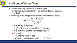
19. Ordinal Variable
 An ordinal variable can be discrete or continuous
 Order is important, e.g., rank
 Can be treated like interval-scaled
 replace xif by their rank
 map the range of each variable onto [0, 1] by replacing
i-th object in the f-th variable by
 compute the dissimilarity using methods for interval-
scaled variables
1
1



f
if
if M
r
z
}
,...,
1
{ f
if
M
r 

20. Attributes of Mixed Type
 A database may contain all attribute types
 Nominal, symmetric binary, asymmetric binary, numeric,
ordinal
 One may use a weighted formula to combine their effects
 f is binary or nominal:
dij
(f) = 0 if xif = xjf , or dij
(f) = 1 otherwise
 f is numeric: use the normalized distance
 f is ordinal
 Compute ranks rif and
 Treat zif as interval-scaled
)
(
1
)
(
)
(
1
)
,
( f
ij
p
f
f
ij
f
ij
p
f
d
j
i
d







1
1



f
if
M
r
zif

21. Cosine Similarity
 A document can be represented by thousands of attributes, each
recording the frequency of a particular word (such as keywords) or
phrase in the document.
 Other vector objects: gene features in micro-arrays, …
 Applications: information retrieval, biologic taxonomy, gene feature
mapping, ...
 Cosine measure: If d1 and d2 are two vectors (e.g., term-frequency
vectors), then
cos(d1, d2) = (d1  d2) /||d1|| ||d2|| ,
where  indicates vector dot product, ||d||: the length of vector d

22. Cosine Similarity Example
 cos(d1, d2) = (d1  d2) /||d1|| ||d2|| ,
where  indicates vector dot product, ||d|: the length of vector d
 Ex: Find the similarity between documents 1 and 2.
d1 = (5, 0, 3, 0, 2, 0, 0, 2, 0, 0)
d2 = (3, 0, 2, 0, 1, 1, 0, 1, 0, 1)
d1d2 = 5*3+0*0+3*2+0*0+2*1+0*1+0*1+2*1+0*0+0*1 = 25
||d1||= (5*5+0*0+3*3+0*0+2*2+0*0+0*0+2*2+0*0+0*0)0.5=(42)0.5 = 6.481
||d2||= (3*3+0*0+2*2+0*0+1*1+1*1+0*0+1*1+0*0+1*1)0.5=(17)0.5 = 4.12
cos(d1, d2 ) = 0.94

23. Measure the Quality of Clustering
 Partitioning criteria
 Single level vs. hierarchical partitioning (often, multi-level hierarchical partitioning
is desirable)
 Separation of clusters
 Exclusive (e.g., one customer belongs to only one region) vs. non-exclusive (e.g.,
one document may belong to more than one class)
 Similarity measure
 Distance-based (e.g., Euclidian, road network, vector) vs. connectivity-based
(e.g., density or contiguity)
 Clustering space
 Full space (often when low dimensional) vs. subspaces (often in high-dimensional
clustering)

24. Requirements and Challenges
 Scalability
 Clustering all the data instead of only on samples
 Ability to deal with different types of attributes
 Numerical, binary, categorical, ordinal, linked, and mixture of
these
 Constraint-based clustering
 User may give inputs on constraints
 Use domain knowledge to determine input parameters
 Interpretability and usability
 Others
 Discovery of clusters with arbitrary shape
 Ability to deal with noisy data
 Incremental clustering and insensitivity to input order
 High dimensionality

25. Major Clustering Approaches
 What are major clustering approaches?
 Partitioning approach:
 Construct various partitions and then evaluate them by some criterion, e.g., minimizing the
sum of square errors
 Typical methods: k-means, k-medoids, CLARANS
 Hierarchical approach:
 Create a hierarchical decomposition of the set of data (or objects) using some criterion
 Typical methods: Diana, Agnes, BIRCH, CAMELEON
 Density-based approach:
 Based on connectivity and density functions
 Typical methods: DBSACN, OPTICS, DenClue
 Grid-based approach:
 based on a multiple-level granularity structure
 Typical methods: STING, WaveCluster, CLIQUE

26. Major Clustering Approaches
 Model-based:
 A model is hypothesized for each of the clusters and tries to find
the best fit of that model to each other
 Typical methods: EM, SOM, COBWEB
 Frequent pattern-based:
 Based on the analysis of frequent patterns
 Typical methods: p-Cluster
 User-guided or constraint-based:
 Clustering by considering user-specified or application-specific
constraints
 Typical methods: COD (obstacles), constrained clustering
 Link-based clustering:
 Objects are often linked together in various ways
 Massive links can be used to cluster objects: SimRank, LinkClus

27. Partitioning Algorithms: Basic Concept
 Partitioning method: Partitioning a database D of n objects into a set of k clusters, such that
the sum of squared distances is minimized (where ci is the centroid or medoid of cluster Ci)
 Given k, find a partition of k clusters that optimizes the chosen partitioning criterion
 Global optimal: exhaustively enumerate all partitions
 Heuristic methods: k-means and k-medoids algorithms
 k-means (MacQueen’67, Lloyd’57/’82): Each cluster is represented by the center of the
cluster
 k-medoids or PAM (Partition around medoids) (Kaufman & Rousseeuw’87): Each cluster
is represented by one of the objects in the cluster
2
1 )
( i
C
p
k
i c
p
E i



 


28. The K-Means Clustering Method
 Given k, the k-means algorithm is implemented in four steps:
 Partition objects into k nonempty subsets
 Compute seed points as the centroids of the clusters of the current
partitioning (the centroid is the center, i.e., mean point, of the cluster)
 Assign each object to the cluster with the nearest seed point
 Go back to Step 2, stop when the assignment does not change

29. An Example of K-Means Clustering
K=2
Arbitrarily
partition
objects into
k groups
Update the
cluster
centroids
Update the
cluster
centroids
Reassign objects
Loop if
needed
The initial data set
 Partition objects into k nonempty
subsets
 Repeat
 Compute centroid (i.e., mean
point) for each partition
 Assign each object to the
cluster of its nearest centroid
 Until no change

30. K-Means Clustering: Example
 Suppose that the data mining task is to cluster points (with (x, y)
representing location) into three clusters, where the points are:
A1 (2,10), A2 (2,5) A3 (8,4), B1(5,8), B2(7,5), B3(6,4), C1(1,2), C2(4,9).
The distance function is Euclidean distance. Suppose initially we assign A1, B1, and
C1 as the center of each cluster, respectively.
 Use the k-means algorithm to show only:
 The three cluster centers after the first round of execution.
 The final three clusters.

31. Comments on the K-Means Method
 Strength: Efficient: O(tkn), where n is # objects, k is # clusters, and t is # iterations.
Normally, k, t << n.
 Comparing: PAM: O(k(n-k)2 ), CLARA: O(ks2 + k(n-k))
 Comment: Often terminates at a local optimal.
 Weakness
 Applicable only to objects in a continuous n-dimensional space
 Using the k-modes method for categorical data
 In comparison, k-medoids can be applied to a wide range of data
 Need to specify k, the number of clusters, in advance (there are ways to
automatically determine the best k (see Hastie et al., 2009)
 Sensitive to noisy data and outliers
 Not suitable to discover clusters with non-convex shapes

32. Variations of the K-Means Method
 Most of the variants of the k-means which differ in
 Selection of the initial k means
 Dissimilarity calculations
 Strategies to calculate cluster means
 Handling categorical data: k-modes
 Replacing means of clusters with modes
 Using new dissimilarity measures to deal with categorical objects
 Using a frequency-based method to update modes of clusters
 A mixture of categorical and numerical data: k-prototype method

33. What is the Problem of the K-Means Method?

34. The K-Medoid Clustering Method
 K-Medoids Clustering: Find representative objects (medoids) in clusters
 PAM (Partitioning Around Medoids, Kaufmann & Rousseeuw 1987)
 Starts from an initial set of medoids and iteratively replaces one of the medoids by
one of the non-medoids if it improves the total distance of the resulting clustering
 PAM works effectively for small data sets, but does not scale well for large data sets
(due to the computational complexity)
 Efficiency improvement on PAM
 CLARA (Kaufmann & Rousseeuw, 1990): PAM on samples
 CLARANS (Ng & Han, 1994): Randomized re-sampling

35. The K-Medoid Clustering Method

36. The K-Medoid Clustering Steps
 Select two medoids randomly.
 Calculate Manhattan distance d from each medoids.
 Assign the data points to the cluster with min distance.
 Calculate the total cost of each cluster.
 Randomly select one non medoid point and swap it with any existing medoids (in previous
iteration) and recalculate the total cost.
 Calculate S, S = Current total cost - Previous total cost
 If S>0 , Hence old clusters are correct.

37. The K- Medoid Clustering Steps
x y
X1 2 6
X2 3 4
X3 3 8
X4 4 7
X5 6 2
X6 6 4
X7 7 3
X8 7 4
X9 8 5
X10 7 6

38. DEPARTMENT OF COMPUTER ENGINEERING, Sanjivani COE, Kopargaon 38
Reference
 Han, Jiawei Kamber, Micheline Pei and Jian, “Data Mining: Concepts and
Techniques”,Elsevier Publishers, ISBN:9780123814791, 9780123814807.
 https://onlinecourses.nptel.ac.in/noc24_cs22