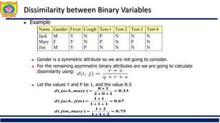
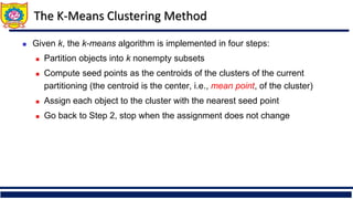
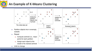
❑ Supervised Vs Unsupervised learning ❑ Clustering/segmentation algorithms-Hierarchical ❑ Distance metrics for categorical data ❑ Distance metrics for continuous ❑ Distance metrics for mixed data ❑ Distance for clusters,k-means clustering ❑ k selection-elbow curve, drawbacks and comparison

1. Sanjivani Rural Education Society’s
Sanjivani College of Engineering, Kopargaon-423 603
(An Autonomous Institute, Affiliated to Savitribai Phule Pune University, Pune)
NACC ‘A’ Grade Accredited, ISO 9001:2015 Certified
Department of Computer Engineering
(NBA Accredited)
Course-CO9301: Unsupervised Modelling for AIML
Unit-III:Unsupervised learning-clustering
Prof. S.A.Shivarkar
Assistant Professor
E-mail : shivarkarsandipcomp@sanjivani.org.in
Contact No: 8275032712

2. ❑ Supervised Vs Unsupervised learning
❑ Clustering/segmentation algorithms-Hierarchical
❑ Distance metrics for categorical data
❑ Distance metrics for continuous
❑ Distance metrics for mixed data
❑ Distance for clusters,k-means clustering
❑ k selection-elbow curve, drawbacks and comparison
Contents

3. What is Cluster Analysis?
◼ Cluster: A collection of data objects
◼ similar (or related) to one another within the same group
◼ dissimilar (or unrelated) to the objects in other groups
◼ Cluster analysis (or clustering, data segmentation, …)
◼ Finding similarities between data according to the
characteristics found in the data and grouping similar
data objects into clusters
◼ Unsupervised learning: no predefined classes (i.e., learning
by observations vs. learning by examples: supervised)
◼ Typical applications
◼ As a stand-alone tool to get insight into data distribution
◼ As a preprocessing step for other algorithms

4. Clustering for Data Understanding and Applications
◼ Biology: taxonomy of living things: kingdom, phylum, class, order, family,
genus and species
◼ Information retrieval: document clustering
◼ Land use: Identification of areas of similar land use in an earth observation
database
◼ Marketing: Help marketers discover distinct groups in their customer bases,
and then use this knowledge to develop targeted marketing programs
◼ City-planning: Identifying groups of houses according to their house type,
value, and geographical location
◼ Earth-quake studies: Observed earth quake epicenters should be clustered
along continent faults
◼ Climate: understanding earth climate, find patterns of atmospheric and ocean
◼ Economic Science: market research

5. Quality: What Is Good Clustering?
◼ A good clustering method will produce high quality
clusters
◼ high intra-class similarity: cohesive within clusters
◼ low inter-class similarity: distinctive between clusters
◼ The quality of a clustering method depends on
◼ the similarity measure used by the method
◼ its implementation, and
◼ Its ability to discover some or all of the hidden patterns

6. Measure the Quality of Clustering
◼ Dissimilarity/Similarity metric
◼ Similarity is expressed in terms of a distance function, typically metric:
d(i, j)
◼ The definitions of distance functions are usually rather different for
interval-scaled, boolean, categorical, ordinal ratio, and vector variables
◼ Weights should be associated with different variables based on
applications and data semantics
◼ Quality of clustering:
◼ There is usually a separate “quality” function that measures the
“goodness” of a cluster.
◼ It is hard to define “similar enough” or “good enough”
◼ The answer is typically highly subjective

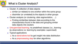
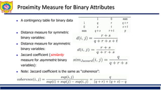
7. Similarity and Dissimilarity
◼ Similarity
◼ Numerical measure of how alike two data objects are
◼ Value is higher when objects are more alike
◼ Often falls in the range [0,1]
◼ Dissimilarity (e.g., distance)
◼ Numerical measure of how different two data objects
are
◼ Lower when objects are more alike
◼ Minimum dissimilarity is often 0
◼ Upper limit varies
◼ Proximity refers to a similarity or dissimilarity

8. Data Matrix and Dissimilarity Matrix
◼ Data matrix
◼ n data points with p
dimensions
◼ Two modes
◼ N by P matrix
◼ Dissimilarity matrix
◼ n data points, but
registers only the
distance
◼ A triangular matrix
◼ Single mode


















np
x
...
nf
x
...
n1
x
...
...
...
...
...
ip
x
...
if
x
...
i1
x
...
...
...
...
...
1p
x
...
1f
x
...
11
x
















0
...
)
2
,
(
)
1
,
(
:
:
:
)
2
,
3
(
)
...
n
d
n
d
0
d
d(3,1
0
d(2,1)
0

9. Proximity Measure for Nominal Attributes
◼ Can take 2 or more states, e.g., red, yellow, blue, green
(generalization of a binary attribute)
◼ Method 1: Simple matching
◼ m: No. of matches, p: total No. of variables
◼ Method 2: Use a large number of binary attributes
◼ creating a new binary attribute for each of the M nominal states
p
m
p
j
i
d −
=
)
,
(

10. Proximity Measure for Binary Attributes
◼ A contingency table for binary data
◼ Distance measure for symmetric
binary variables:
◼ Distance measure for asymmetric
binary variables:
◼ Jaccard coefficient (similarity
measure for asymmetric binary
variables):
◼ Note: Jaccard coefficient is the same as “coherence”:

11. Dissimilarity between Binary Variables
◼ Example
◼ Gender is a symmetric attribute so we are not going to consider.
◼ For the remaining asymmetric binary attributes are we are going to calculate
dissimilarity using:
◼ Let the values Y and P be 1, and the value N 0
Name Gender Fever Cough Test-1 Test-2 Test-3 Test-4
Jack M Y N P N N N
Mary F Y N P N P N
Jim M Y P N N N N
75
.
0
2
1
1
2
1
)
,
(
67
.
0
1
1
1
1
1
)
,
(
33
.
0
1
0
2
1
0
)
,
(
=
+
+
+
=
=
+
+
+
=
=
+
+
+
=
mary
jim
d
jim
jack
d
mary
jack
d

12. Standardizing Numeric Data
◼ Numeric data is biased, it may varies in range e.g. 1,100,100000.
◼ So needs to normalize it.
◼ Z-score:
◼ X: raw score to be standardized, μ: mean of the population, σ: standard
deviation
◼ the distance between the raw score and the population mean in units of the
standard deviation
◼ negative when the raw score is below the mean, “+” when above
◼ An alternative way: Calculate the mean absolute deviation
where
◼ standardized measure (z-score):
◼ Using mean absolute deviation is more robust than using standard deviation
.
)
...
2
1
1
nf
f
f
f
x
x
(x
n
m +
+
+
=
|)
|
...
|
|
|
(|
1
2
1 f
nf
f
f
f
f
f
m
x
m
x
m
x
n
s −
+
+
−
+
−
=
f
f
if
if s
m
x
z
−
=


−
= x
z

13. Example: Data Matrix and Dissimilarity Matrix
point attribute1 attribute2
x1 1 2
x2 3 5
x3 2 0
x4 4 5
Dissimilarity Matrix
(with Euclidean Distance)
x1 x2 x3 x4
x1 0
x2 3.61 0
x3 5.1 5.1 0
x4 4.24 1 5.39 0
Data Matrix

14. Distance on Numeric Data: Minkowski Distance
◼ Minkowski distance: A popular distance measure
where i = (xi1, xi2, …, xip) and j = (xj1, xj2, …, xjp) are two p-dimensional
data objects, and h is the order (the distance so defined is also called
L-h norm)
◼ Properties
◼ d(i, j) > 0 if i ≠ j, and d(i, i) = 0 (Positive definiteness)
◼ d(i, j) = d(j, i) (Symmetry)
◼ d(i, j)  d(i, k) + d(k, j) (Triangle Inequality)
◼ A distance that satisfies these properties is a metric

15. Special Cases of Minkowski Distance
◼ h = 1: Manhattan (city block, L1 norm) distance
◼ E.g., the Hamming distance: the number of bits that are different between
two binary vectors
◼ h = 2: (L2 norm) Euclidean distance
◼ h → . “supremum” (Lmax norm, L norm) distance.
◼ This is the maximum difference between any component (attribute) of the
vectors
)
|
|
...
|
|
|
(|
)
,
( 2
2
2
2
2
1
1 p
p j
x
i
x
j
x
i
x
j
x
i
x
j
i
d −
+
+
−
+
−
=
|
|
...
|
|
|
|
)
,
(
2
2
1
1 p
p j
x
i
x
j
x
i
x
j
x
i
x
j
i
d −
+
+
−
+
−
=

16. Special Cases of Minkowski Distance
◼ h = 1: Manhattan (city block, L1 norm) distance
◼ E.g., the Hamming distance: the number of bits that are different between
two binary vectors
◼ h = 2: (L2 norm) Euclidean distance
◼ h → . “supremum” (Lmax norm, L norm) distance.
◼ This is the maximum difference between any component (attribute) of the
vectors
)
|
|
...
|
|
|
(|
)
,
( 2
2
2
2
2
1
1 p
p j
x
i
x
j
x
i
x
j
x
i
x
j
i
d −
+
+
−
+
−
=
|
|
...
|
|
|
|
)
,
(
2
2
1
1 p
p j
x
i
x
j
x
i
x
j
x
i
x
j
i
d −
+
+
−
+
−
=

17. Example of Minkowski Distance
Dissimilarity Matrices
point attribute 1 attribute 2
x1 1 2
x2 3 5
x3 2 0
x4 4 5
L x1 x2 x3 x4
x1 0
x2 5 0
x3 3 6 0
x4 6 1 7 0
L2 x1 x2 x3 x4
x1 0
x2 3.61 0
x3 2.24 5.1 0
x4 4.24 1 5.39 0
L x1 x2 x3 x4
x1 0
x2 3 0
x3 2 5 0
x4 3 1 5 0
Manhattan (L1)
Euclidean (L2)
Supremum

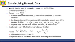
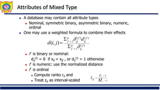
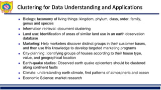
18. Ordinal Variable
◼ An ordinal variable can be discrete or continuous
◼ Order is important, e.g., rank
◼ Can be treated like interval-scaled
◼ replace xif by their rank
◼ map the range of each variable onto [0, 1] by replacing
i-th object in the f-th variable by
◼ compute the dissimilarity using methods for interval-
scaled variables
1
1
−
−
=
f
if
if M
r
z
}
,...,
1
{ f
if
M
r 

19. Attributes of Mixed Type
◼ A database may contain all attribute types
◼ Nominal, symmetric binary, asymmetric binary, numeric,
ordinal
◼ One may use a weighted formula to combine their effects
◼ f is binary or nominal:
dij
(f) = 0 if xif = xjf , or dij
(f) = 1 otherwise
◼ f is numeric: use the normalized distance
◼ f is ordinal
◼ Compute ranks rif and
◼ Treat zif as interval-scaled
)
(
1
)
(
)
(
1
)
,
( f
ij
p
f
f
ij
f
ij
p
f
d
j
i
d


=
=


=
1
1
−
−
=
f
if
M
r
zif

20. Cosine Similarity
◼ A document can be represented by thousands of attributes, each
recording the frequency of a particular word (such as keywords) or
phrase in the document.
◼ Other vector objects: gene features in micro-arrays, …
◼ Applications: information retrieval, biologic taxonomy, gene feature
mapping, ...
◼ Cosine measure: If d1 and d2 are two vectors (e.g., term-frequency
vectors), then
cos(d1, d2) = (d1 • d2) /||d1|| ||d2|| ,
where • indicates vector dot product, ||d||: the length of vector d

21. Cosine Similarity Example
◼ cos(d1, d2) = (d1 • d2) /||d1|| ||d2|| ,
where • indicates vector dot product, ||d|: the length of vector d
◼ Ex: Find the similarity between documents 1 and 2.
d1 = (5, 0, 3, 0, 2, 0, 0, 2, 0, 0)
d2 = (3, 0, 2, 0, 1, 1, 0, 1, 0, 1)
d1•d2 = 5*3+0*0+3*2+0*0+2*1+0*1+0*1+2*1+0*0+0*1 = 25
||d1||= (5*5+0*0+3*3+0*0+2*2+0*0+0*0+2*2+0*0+0*0)0.5=(42)0.5 = 6.481
||d2||= (3*3+0*0+2*2+0*0+1*1+1*1+0*0+1*1+0*0+1*1)0.5=(17)0.5 =
4.12
cos(d1, d2 ) = 0.94

22. Measure the Quality of Clustering
◼ Partitioning criteria
◼ Single level vs. hierarchical partitioning (often, multi-level hierarchical partitioning
is desirable)
◼ Separation of clusters
◼ Exclusive (e.g., one customer belongs to only one region) vs. non-exclusive (e.g.,
one document may belong to more than one class)
◼ Similarity measure
◼ Distance-based (e.g., Euclidian, road network, vector) vs. connectivity-based
(e.g., density or contiguity)
◼ Clustering space
◼ Full space (often when low dimensional) vs. subspaces (often in high-dimensional
clustering)

23. Requirements and Challenges
◼ Scalability
◼ Clustering all the data instead of only on samples
◼ Ability to deal with different types of attributes
◼ Numerical, binary, categorical, ordinal, linked, and mixture of
these
◼ Constraint-based clustering
◼ User may give inputs on constraints
◼ Use domain knowledge to determine input parameters
◼ Interpretability and usability
◼ Others
◼ Discovery of clusters with arbitrary shape
◼ Ability to deal with noisy data
◼ Incremental clustering and insensitivity to input order
◼ High dimensionality

24. Major Clustering Approaches
◼ What are major clustering approaches?
◼ Partitioning approach:
◼ Construct various partitions and then evaluate them by some criterion, e.g., minimizing the
sum of square errors
◼ Typical methods: k-means, k-medoids, CLARANS
◼ Hierarchical approach:
◼ Create a hierarchical decomposition of the set of data (or objects) using some criterion
◼ Typical methods: Diana, Agnes, BIRCH, CAMELEON
◼ Density-based approach:
◼ Based on connectivity and density functions
◼ Typical methods: DBSACN, OPTICS, DenClue
◼ Grid-based approach:
◼ based on a multiple-level granularity structure
◼ Typical methods: STING, WaveCluster, CLIQUE

25. Major Clustering Approaches
◼ Model-based:
◼ A model is hypothesized for each of the clusters and tries to find
the best fit of that model to each other
◼ Typical methods: EM, SOM, COBWEB
◼ Frequent pattern-based:
◼ Based on the analysis of frequent patterns
◼ Typical methods: p-Cluster
◼ User-guided or constraint-based:
◼ Clustering by considering user-specified or application-specific
constraints
◼ Typical methods: COD (obstacles), constrained clustering
◼ Link-based clustering:
◼ Objects are often linked together in various ways
◼ Massive links can be used to cluster objects: SimRank, LinkClus

26. Partitioning Algorithms: Basic Concept
◼ Partitioning method: Partitioning a database D of n objects into a set of k clusters, such that
the sum of squared distances is minimized (where ci is the centroid or medoid of cluster Ci)
◼ Given k, find a partition of k clusters that optimizes the chosen partitioning criterion
◼ Global optimal: exhaustively enumerate all partitions
◼ Heuristic methods: k-means and k-medoids algorithms
◼ k-means (MacQueen’67, Lloyd’57/’82): Each cluster is represented by the center of the
cluster
◼ k-medoids or PAM (Partition around medoids) (Kaufman & Rousseeuw’87): Each cluster
is represented by one of the objects in the cluster
2
1 )
( i
C
p
k
i c
p
E i
−


= 
=

27. The K-Means Clustering Method
◼ Given k, the k-means algorithm is implemented in four steps:
◼ Partition objects into k nonempty subsets
◼ Compute seed points as the centroids of the clusters of the current
partitioning (the centroid is the center, i.e., mean point, of the cluster)
◼ Assign each object to the cluster with the nearest seed point
◼ Go back to Step 2, stop when the assignment does not change

28. An Example of K-Means Clustering
K=2
Arbitrarily
partition
objects into
k groups
Update the
cluster
centroids
Update the
cluster
centroids
Reassign objects
Loop if
needed
The initial data set
◼ Partition objects into k nonempty
subsets
◼ Repeat
◼ Compute centroid (i.e., mean
point) for each partition
◼ Assign each object to the
cluster of its nearest centroid
◼ Until no change

29. K-Means Clustering: Example
◼ Suppose that the data mining task is to cluster points (with (x, y)
representing location) into three clusters, where the points are:
A1 (2,10), A2 (2,5) A3 (8,4), B1(5,8), B2(7,5), B3(6,4), C1(1,2), C2(4,9).
The distance function is Euclidean distance. Suppose initially we assign A1, B1, and
C1 as the center of each cluster, respectively.
◼ Use the k-means algorithm to show only:
◼The three cluster centers after the first round of execution.
◼The final three clusters.

30. Comments on the K-Means Method
◼ Strength: Efficient: O(tkn), where n is # objects, k is # clusters, and t is # iterations.
Normally, k, t << n.
◼ Comparing: PAM: O(k(n-k)2 ), CLARA: O(ks2 + k(n-k))
◼ Comment: Often terminates at a local optimal.
◼ Weakness
◼ Applicable only to objects in a continuous n-dimensional space
◼ Using the k-modes method for categorical data
◼ In comparison, k-medoids can be applied to a wide range of data
◼ Need to specify k, the number of clusters, in advance (there are ways to
automatically determine the best k (see Hastie et al., 2009)
◼ Sensitive to noisy data and outliers
◼ Not suitable to discover clusters with non-convex shapes

31. Variations of the K-Means Method
◼ Most of the variants of the k-means which differ in
◼ Selection of the initial k means
◼ Dissimilarity calculations
◼ Strategies to calculate cluster means
◼ Handling categorical data: k-modes
◼ Replacing means of clusters with modes
◼ Using new dissimilarity measures to deal with categorical objects
◼ Using a frequency-based method to update modes of clusters
◼ A mixture of categorical and numerical data: k-prototype method

32. What is the Problem of the K-Means Method?

33. The K-Medoid Clustering Method
◼ K-Medoids Clustering: Find representative objects (medoids) in clusters
◼ PAM (Partitioning Around Medoids, Kaufmann & Rousseeuw 1987)
◼ Starts from an initial set of medoids and iteratively replaces one of the medoids by
one of the non-medoids if it improves the total distance of the resulting clustering
◼ PAM works effectively for small data sets, but does not scale well for large data sets
(due to the computational complexity)
◼ Efficiency improvement on PAM
◼ CLARA (Kaufmann & Rousseeuw, 1990): PAM on samples
◼ CLARANS (Ng & Han, 1994): Randomized re-sampling

34. The K-Medoid Clustering Method

35. The K-Medoid Clustering Steps
◼ Select two medoids randomly.
◼ Calculate Manhattan distance d from each medoids.
◼ Assign the data points to the cluster with min distance.
◼ Calculate the total cost of each cluster.
◼ Randomly select one non medoid point and swap it with any existing medoids (in previous
iteration) and recalculate the total cost.
◼ Calculate S, S = Current total cost - Previous total cost
◼ If S>0 , Hence old clusters are correct.

36. The K- Medoid Clustering Steps
x y
X1 2 6
X2 3 4
X3 3 8
X4 4 7
X5 6 2
X6 6 4
X7 7 3
X8 7 4
X9 8 5
X10 7 6

37. DEPARTMENT OF COMPUTER ENGINEERING, Sanjivani COE, Kopargaon 37
Reference
❖ Han, Jiawei Kamber, Micheline Pei and Jian, “Data Mining: Concepts and
Techniques”,Elsevier Publishers, ISBN:9780123814791, 9780123814807.
❖ https://onlinecourses.nptel.ac.in/noc24_cs22

38. DEPARTMENT OF COMPUTER ENGINEERING, Sanjivani COE, Kopargaon 38
Thank You