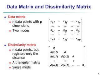
This document discusses various techniques for analyzing and visualizing data to gain insights. It covers data attribute types, basic statistical descriptions to understand data distribution and outliers, different visualization methods to discover patterns and relationships, and various ways to measure similarity between data objects, including distances, coefficients, and cosine similarity for text. The goal is to preprocess and understand data at a high level before applying more advanced analytics.

1. 1
Data Mining:
Concepts and Techniques
— Chapter 2 —
Jiawei Han, Micheline Kamber, and Jian Pei
University of Illinois at Urbana-Champaign
Simon Fraser University
©2011 Han, Kamber, and Pei. All rights reserved.

2. 2
Chapter 2: Getting to Know Your Data
 Data Objects and Attribute Types
 Basic Statistical Descriptions of Data
 Data Visualization
 Measuring Data Similarity and Dissimilarity
 Summary

3. 3
Data Visualization
 Why data visualization?
 Gain insight into an information space by mapping data onto graphical
primitives
 Provide qualitative overview of large data sets
 Search for patterns, trends, structure, irregularities, relationships among
data
 Help find interesting regions and suitable parameters for further
quantitative analysis
 Provide a visual proof of computer representations derived
 Categorization of visualization methods:
 Pixel-oriented visualization techniques
 Geometric projection visualization techniques
 Icon-based visualization techniques
 Hierarchical visualization techniques
 Visualizing complex data and relations

4. 4
Chapter 2: Getting to Know Your Data
 Data Objects and Attribute Types
 Basic Statistical Descriptions of Data
 Data Visualization
 Measuring Data Similarity and Dissimilarity
 Summary

5. 5
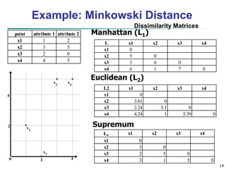
Similarity and Dissimilarity
 Similarity
 Numerical measure of how alike two data objects are
 Value is higher when objects are more alike
 Often falls in the range [0,1]
 Dissimilarity (e.g., distance)
 Numerical measure of how different two data objects
are
 Lower when objects are more alike
 Minimum dissimilarity is often 0
 Upper limit varies
 Proximity refers to a similarity or dissimilarity

6. 6
Data Matrix and Dissimilarity Matrix
 Data matrix
 n data points with p
dimensions
 Two modes
 Dissimilarity matrix
 n data points, but
registers only the
distance
 A triangular matrix
 Single mode


















np
x
...
nf
x
...
n1
x
...
...
...
...
...
ip
x
...
if
x
...
i1
x
...
...
...
...
...
1p
x
...
1f
x
...
11
x
















0
...
)
2
,
(
)
1
,
(
:
:
:
)
2
,
3
(
)
...
n
d
n
d
0
d
d(3,1
0
d(2,1)
0

7. 7
Proximity Measure for Nominal Attributes
 Can take 2 or more states, e.g., red, yellow, blue,
green (generalization of a binary attribute)
 Method 1: Simple matching
 m: # of matches, p: total # of variables
 Method 2: Use a large number of binary attributes
 creating a new binary attribute for each of the
M nominal states
p
m
p
j
i
d 

)
,
(

8. 8
Proximity Measure for Binary Attributes
 A contingency table for binary data
 Distance measure for symmetric
binary variables:
 Distance measure for asymmetric
binary variables:
 Jaccard coefficient (similarity
measure for asymmetric binary
variables):
 Note: Jaccard coefficient is the same as “coherence”:
Object i
Object j

9. 9
Dissimilarity between Binary Variables
 Example
 Gender is a symmetric attribute
 The remaining attributes are asymmetric binary
 Let the values Y and P be 1, and the value N 0
Name Gender Fever Cough Test-1 Test-2 Test-3 Test-4
Jack M Y N P N N N
Mary F Y N P N P N
Jim M Y P N N N N
75
.
0
2
1
1
2
1
)
,
(
67
.
0
1
1
1
1
1
)
,
(
33
.
0
1
0
2
1
0
)
,
(















mary
jim
d
jim
jack
d
mary
jack
d

10. 10
Standardizing Numeric Data
 Z-score:
 X: raw score to be standardized, μ: mean of the population, σ:
standard deviation
 the distance between the raw score and the population mean in
units of the standard deviation
 negative when the raw score is below the mean, “+” when above
 An alternative way: Calculate the mean absolute deviation
where
 standardized measure (z-score):
 Using mean absolute deviation is more robust than using standard
deviation
.
)
...
2
1
1
nf
f
f
f
x
x
(x
n
m 



|)
|
...
|
|
|
(|
1
2
1 f
nf
f
f
f
f
f
m
x
m
x
m
x
n
s 






f
f
if
if s
m
x
z





 x
z

11. 11
Example:
Data Matrix and Dissimilarity Matrix
point attribute1 attribute2
x1 1 2
x2 3 5
x3 2 0
x4 4 5
Dissimilarity Matrix
(with Euclidean Distance)
x1 x2 x3 x4
x1 0
x2 3.61 0
x3 5.1 5.1 0
x4 4.24 1 5.39 0
Data Matrix

12. 12
Distance on Numeric Data: Minkowski
Distance
 Minkowski distance: A popular distance measure
where i = (xi1, xi2, …, xip) and j = (xj1, xj2, …, xjp) are two
p-dimensional data objects, and h is the order (the
distance so defined is also called L-h norm)
 Properties
 d(i, j) > 0 if i ≠ j, and d(i, i) = 0 (Positive definiteness)
 d(i, j) = d(j, i) (Symmetry)
 d(i, j)  d(i, k) + d(k, j) (Triangle Inequality)
 A distance that satisfies these properties is a metric

13. 13
Special Cases of Minkowski Distance
 h = 1: Manhattan (city block, L1 norm) distance
 E.g., the Hamming distance: the number of bits that are
different between two binary vectors
 h = 2: (L2 norm) Euclidean distance
 h  . “supremum” (Lmax norm, L norm) distance.
 This is the maximum difference between any component
(attribute) of the vectors
)
|
|
...
|
|
|
(|
)
,
( 2
2
2
2
2
1
1 p
p j
x
i
x
j
x
i
x
j
x
i
x
j
i
d 






|
|
...
|
|
|
|
)
,
(
2
2
1
1 p
p j
x
i
x
j
x
i
x
j
x
i
x
j
i
d 







14. 14
Example: Minkowski Distance
Dissimilarity Matrices
point attribute 1 attribute 2
x1 1 2
x2 3 5
x3 2 0
x4 4 5
L x1 x2 x3 x4
x1 0
x2 5 0
x3 3 6 0
x4 6 1 7 0
L2 x1 x2 x3 x4
x1 0
x2 3.61 0
x3 2.24 5.1 0
x4 4.24 1 5.39 0
L x1 x2 x3 x4
x1 0
x2 3 0
x3 2 5 0
x4 3 1 5 0
Manhattan (L1)
Euclidean (L2)
Supremum

15. 15
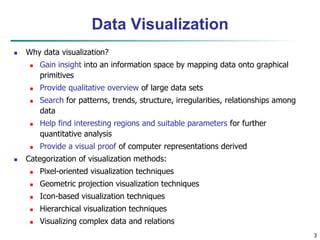
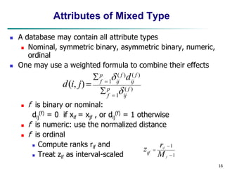
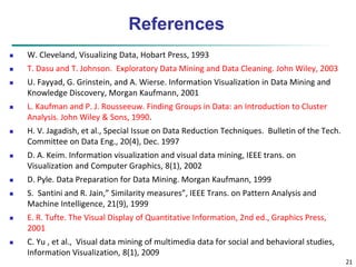
Ordinal Variables
 An ordinal variable can be discrete or continuous
 Order is important, e.g., rank
 Can be treated like interval-scaled
 replace xif by their rank
 map the range of each variable onto [0, 1] by replacing
i-th object in the f-th variable by
 compute the dissimilarity using methods for interval-
scaled variables
1
1



f
if
if M
r
z
}
,...,
1
{ f
if
M
r 

16. 16
Attributes of Mixed Type
 A database may contain all attribute types
 Nominal, symmetric binary, asymmetric binary, numeric,
ordinal
 One may use a weighted formula to combine their effects
 f is binary or nominal:
dij
(f) = 0 if xif = xjf , or dij
(f) = 1 otherwise
 f is numeric: use the normalized distance
 f is ordinal
 Compute ranks rif and
 Treat zif as interval-scaled
)
(
1
)
(
)
(
1
)
,
( f
ij
p
f
f
ij
f
ij
p
f
d
j
i
d







1
1



f
if
M
r
zif

17. 17
Cosine Similarity
 A document can be represented by thousands of attributes, each
recording the frequency of a particular word (such as keywords) or
phrase in the document.
 Other vector objects: gene features in micro-arrays, …
 Applications: information retrieval, biologic taxonomy, gene feature
mapping, ...
 Cosine measure: If d1 and d2 are two vectors (e.g., term-frequency
vectors), then
cos(d1, d2) = (d1  d2) /||d1|| ||d2|| ,
where  indicates vector dot product, ||d||: the length of vector d

18. 18
Example: Cosine Similarity
 cos(d1, d2) = (d1  d2) /||d1|| ||d2|| ,
where  indicates vector dot product, ||d|: the length of vector d
 Ex: Find the similarity between documents 1 and 2.
d1 = (5, 0, 3, 0, 2, 0, 0, 2, 0, 0)
d2 = (3, 0, 2, 0, 1, 1, 0, 1, 0, 1)
d1d2 = 5*3+0*0+3*2+0*0+2*1+0*1+0*1+2*1+0*0+0*1 = 25
||d1||= (5*5+0*0+3*3+0*0+2*2+0*0+0*0+2*2+0*0+0*0)0.5=(42)0.5
= 6.481
||d2||= (3*3+0*0+2*2+0*0+1*1+1*1+0*0+1*1+0*0+1*1)0.5=(17)0.5
= 4.12
cos(d1, d2 ) = 0.94

19. 19
Chapter 2: Getting to Know Your Data
 Data Objects and Attribute Types
 Basic Statistical Descriptions of Data
 Data Visualization
 Measuring Data Similarity and Dissimilarity
 Summary

20. Summary
 Data attribute types: nominal, binary, ordinal, interval-scaled, ratio-
scaled
 Many types of data sets, e.g., numerical, text, graph, Web, image.
 Gain insight into the data by:
 Basic statistical data description: central tendency, dispersion,
graphical displays
 Data visualization: map data onto graphical primitives
 Measure data similarity
 Above steps are the beginning of data preprocessing.
 Many methods have been developed but still an active area of research.
20

21. References
 W. Cleveland, Visualizing Data, Hobart Press, 1993
 T. Dasu and T. Johnson. Exploratory Data Mining and Data Cleaning. John Wiley, 2003
 U. Fayyad, G. Grinstein, and A. Wierse. Information Visualization in Data Mining and
Knowledge Discovery, Morgan Kaufmann, 2001
 L. Kaufman and P. J. Rousseeuw. Finding Groups in Data: an Introduction to Cluster
Analysis. John Wiley & Sons, 1990.
 H. V. Jagadish, et al., Special Issue on Data Reduction Techniques. Bulletin of the Tech.
Committee on Data Eng., 20(4), Dec. 1997
 D. A. Keim. Information visualization and visual data mining, IEEE trans. on
Visualization and Computer Graphics, 8(1), 2002
 D. Pyle. Data Preparation for Data Mining. Morgan Kaufmann, 1999
 S. Santini and R. Jain,” Similarity measures”, IEEE Trans. on Pattern Analysis and
Machine Intelligence, 21(9), 1999
 E. R. Tufte. The Visual Display of Quantitative Information, 2nd ed., Graphics Press,
2001
 C. Yu , et al., Visual data mining of multimedia data for social and behavioral studies,
Information Visualization, 8(1), 2009
21