This document provides an overview of clustering evaluation and practical issues in advanced data mining. It discusses both extrinsic and intrinsic evaluation of clustering results using measures like purity, normalized mutual information, precision, recall, and silhouette coefficient. It also covers similarity and dissimilarity measures for different data types, including numeric, binary, and mixed attribute data. Standardization techniques for numeric data and distance measures like Minkowski and cosine similarity are also summarized.

1. CS249: ADVANCED DATA MINING
Instructor: Yizhou Sun
yzsun@cs.ucla.edu
May 2, 2017
Clustering Evaluation and Practical Issues

2. Announcements
•Homework 2 due later today
• Due May 3rd (11:59pm)
•Course project proposal
• Due May 8th (11:59pm)
•Homework 3 out
• Due May 10th (11:59pm)
2

3. Learnt Clustering Methods
3
Vector Data Text Data Recommender
System
Graph & Network
Classification Decision Tree; Naïve
Bayes; Logistic
Regression
SVM; NN
Label Propagation
Clustering K-means; hierarchical
clustering; DBSCAN;
Mixture Models;
kernel k-means
PLSA;
LDA
Matrix Factorization SCAN; Spectral
Clustering
Prediction Linear Regression
GLM
Collaborative Filtering
Ranking PageRank
Feature
Representation
Word embedding Network embedding

4. Evaluation and Other Practical Issues
•Evaluation of Clustering
•Similarity and Dissimilarity
•Summary
4

5. Measuring Clustering Quality
• Two methods: extrinsic vs. intrinsic
• Extrinsic: supervised, i.e., the ground truth is available
• Compare a clustering against the ground truth using certain
clustering quality measure
• Ex. Purity, precision and recall metrics, normalized mutual
information
• Intrinsic: unsupervised, i.e., the ground truth is unavailable
• Evaluate the goodness of a clustering by considering how well
the clusters are separated, and how compact the clusters are
• Ex. Silhouette coefficient
5

6. Purity
• Let 𝑪𝑪 = 𝑐𝑐1, … , 𝑐𝑐𝐾𝐾 be the output clustering
result, 𝜴𝜴 = 𝜔𝜔1, … , 𝜔𝜔𝐽𝐽 be the ground truth
clustering result (ground truth class)
• 𝑐𝑐𝑘𝑘 𝑎𝑎𝑎𝑎𝑎𝑎 𝑤𝑤𝑘𝑘 are sets of data points
• 𝑝𝑝𝑝𝑝𝑝𝑝𝑝𝑝𝑝𝑝𝑝𝑝 𝐶𝐶, Ω =
1
𝑁𝑁
∑𝑘𝑘 max
𝑗𝑗
|𝑐𝑐𝑘𝑘 ∩ 𝜔𝜔𝑗𝑗|
6

7. Example
• Clustering output: cluster 1, cluster 2, and cluster 3
• Ground truth clustering result: ×’s, ◊’s, and ○’s.
• cluster 1 vs. ×’s, cluster 2 vs. ○’s, and cluster 3 vs. ◊’s
7

8. Normalized Mutual Information
• 𝑁𝑁𝑁𝑁𝑁𝑁 𝐶𝐶, Ω =
𝐼𝐼(𝐶𝐶,Ω)
𝐻𝐻 𝐶𝐶 𝐻𝐻(Ω)
• 𝐼𝐼 Ω, 𝐶𝐶 = ∑𝑘𝑘 ∑𝑗𝑗 𝑃𝑃(𝑐𝑐𝑘𝑘 ∩ 𝜔𝜔𝑗𝑗) 𝑙𝑙𝑙𝑙𝑙𝑙
𝑃𝑃(𝑐𝑐𝑘𝑘∩𝑤𝑤𝑗𝑗)
𝑃𝑃 𝑐𝑐𝑘𝑘 𝑃𝑃(𝑤𝑤𝑗𝑗)
• 𝐻𝐻 Ω = − ∑𝑗𝑗 𝑃𝑃 𝑤𝑤𝑗𝑗 𝑙𝑙𝑙𝑙𝑙𝑙𝑙𝑙 𝑤𝑤𝑗𝑗
= − �
𝑗𝑗
|𝜔𝜔𝑗𝑗|
𝑁𝑁
𝑙𝑙𝑙𝑙𝑙𝑙
|𝜔𝜔𝑗𝑗|
𝑁𝑁
8
= ∑𝑘𝑘 ∑𝑗𝑗
|𝑐𝑐𝑘𝑘∩𝜔𝜔𝑗𝑗|
𝑁𝑁
𝑙𝑙𝑙𝑙𝑙𝑙
𝑁𝑁|𝑐𝑐𝑘𝑘∩𝜔𝜔𝑗𝑗|
𝑐𝑐𝑘𝑘 ⋅|𝑤𝑤𝑗𝑗|

9. Example
Cluster 1 Cluster 2 Cluster 3 sum
crosses 5 1 2 8
circles 1 4 0 5
diamonds 0 1 3 4
sum 6 6 5 N=17
9
|𝝎𝝎𝒌𝒌 ∩ 𝒄𝒄𝒋𝒋| |𝝎𝝎𝒌𝒌|
|𝒄𝒄𝒋𝒋|
NMI=0.36

10. Precision and Recall
• Random Index (RI) = (TP+TN)/(TP+FP+FN+TN)
• F-measure: 2P*R/(P+R)
• P = TP/(TP+FP)
• R = TP/(TP+FN)
• Consider pairs of data points:
• hopefully, two data points that are in the same cluster will be
clustered into the same cluster (TP), and two data points that are
in different clusters will be clustered into different clusters (TN).
10
Same cluster Different clusters
Same class TP FN
Different classes FP TN

11. Example
Data points Output clustering Ground truth
clustering (class)
a 1 2
b 1 2
c 2 2
d 2 1
11
• # pairs of data points: 6
• (a, b): same class, same cluster
• (a, c): same class, different cluster
• (a, d): different class, different cluster
• (b, c): same class, different cluster
• (b, d): different class, different cluster
• (c, d): different class, same cluster
TP = 1
FP = 1
FN = 2
TN = 2
RI = 0.5
P= ½, R= 1/3, F = 0.4

12. Question
•If we flip the ground truth cluster labels
(2->1 and 1->2), will the evaluation results
be the same?
12
Data points Output clustering Ground truth
clustering (class)
a 1 2
b 1 2
c 2 2
d 2 1

13. Evaluation and Other Practical Issues
•Evaluation of Clustering
•Similarity and Dissimilarity
•Summary
13

14. Similarity and Dissimilarity
• Similarity
• Numerical measure of how alike two data objects are
• Value is higher when objects are more alike
• Often falls in the range [0,1]
• Dissimilarity (e.g., distance)
• Numerical measure of how different two data objects are
• Lower when objects are more alike
• Minimum dissimilarity is often 0
• Upper limit varies
• Proximity refers to a similarity or dissimilarity
14

15. Data Matrix and Dissimilarity Matrix
• Data matrix
• n data points with p
dimensions
• Two modes
• Dissimilarity matrix
• n data points, but registers
only the distance
• A triangular matrix
• Single mode
15


















np
x
...
nf
x
...
n1
x
...
...
...
...
...
ip
x
...
if
x
...
i1
x
...
...
...
...
...
1p
x
...
1f
x
...
11
x
















0
...
)
2
,
(
)
1
,
(
:
:
:
)
2
,
3
(
)
...
n
d
n
d
0
d
d(3,1
0
d(2,1)
0

16. Example:
DataMatrixandDissimilarityMatrix
16
point attribute1 attribute2
x1 1 2
x2 3 5
x3 2 0
x4 4 5
Dissimilarity Matrix
(with Euclidean Distance)
x1 x2 x3 x4
x1 0
x2 3.61 0
x3 2.24 5.1 0
x4 4.24 1 5.39 0
Data Matrix
0 2 4
2
4
x
1
x
2
x
3
x
4

17. Proximity Measure for Nominal Attributes
• Can take 2 or more states, e.g., red, yellow, blue, green
(generalization of a binary attribute)
• Method 1: Simple matching
• m: # of matches, p: total # of variables
• Method 2: Use a large number of binary attributes
• creating a new binary attribute for each of the M nominal states
17
p
m
p
j
i
d −
=
)
,
(

18. Proximity Measure for Binary Attributes
• A contingency table for binary data
• Distance measure for symmetric binary
variables:
• Distance measure for asymmetric binary
variables:
• Jaccard coefficient (similarity measure
for asymmetric binary variables):
Object i
Object j
18

19. Dissimilarity between Binary Variables
• Example
• Gender is a symmetric attribute
• The remaining attributes are asymmetric binary
• Let the values Y and P be 1, and the value N be 0
19
Name Gender Fever Cough Test-1 Test-2 Test-3 Test-4
Jack M Y N P N N N
Mary F Y N P N P N
Jim M Y P N N N N
75
.
0
2
1
1
2
1
)
,
(
67
.
0
1
1
1
1
1
)
,
(
33
.
0
1
0
2
1
0
)
,
(
=
+
+
+
=
=
+
+
+
=
=
+
+
+
=
mary
jim
d
jim
jack
d
mary
jack
d

20. Standardizing Numeric Data
• Z-score:
• X: raw score to be standardized, μ: mean of the population, σ: standard
deviation
• the distance between the raw score and the population mean in units of
the standard deviation
• negative when the raw score is below the mean, “+” when above
• An alternative way: Calculate the mean absolute deviation
where
• standardized measure (z-score):
• Using mean absolute deviation is more robust than using standard deviation
σ
µ
−
= x
z
.
)
...
2
1
1
nf
f
f
f
x
x
(x
n
m +
+
+
=
|)
|
...
|
|
|
(|
1
2
1 f
nf
f
f
f
f
f
m
x
m
x
m
x
n
s −
+
+
−
+
−
=
f
f
if
if s
m
x
z
−
=
20

21. Distance on Numeric Data: Minkowski Distance
• Minkowski distance: A popular distance measure
where i = (xi1, xi2, …, xip) and j = (xj1, xj2, …, xjp) are two p-
dimensional data objects, and h is the order (the distance so
defined is also called L-h norm)
• Properties
• d(i, j) > 0 if i ≠ j, and d(i, i) = 0 (Positive definiteness)
• d(i, j) = d(j, i) (Symmetry)
• d(i, j) ≤ d(i, k) + d(k, j) (Triangle Inequality)
• A distance that satisfies these properties is a metric
21

22. Special Cases of Minkowski Distance
• h = 1: Manhattan (city block, L1 norm) distance
• E.g., the Hamming distance: the number of bits that are different
between two binary vectors
• h = 2: (L2 norm) Euclidean distance
• h → ∞. “supremum” (Lmax norm, L∞ norm) distance.
• This is the maximum difference between any component
(attribute) of the vectors
|
|
...
|
|
|
|
)
,
(
2
2
1
1 p
p j
x
i
x
j
x
i
x
j
x
i
x
j
i
d −
+
+
−
+
−
=
22
)
|
|
...
|
|
|
(|
)
,
( 2
2
2
2
2
1
1 p
p j
x
i
x
j
x
i
x
j
x
i
x
j
i
d −
+
+
−
+
−
=

23. Example: Minkowski Distance
23
Dissimilarity Matrices
point attribute 1 attribute 2
x1 1 2
x2 3 5
x3 2 0
x4 4 5
L x1 x2 x3 x4
x1 0
x2 5 0
x3 3 6 0
x4 6 1 7 0
L2 x1 x2 x3 x4
x1 0
x2 3.61 0
x3 2.24 5.1 0
x4 4.24 1 5.39 0
L∞ x1 x2 x3 x4
x1 0
x2 3 0
x3 2 5 0
x4 3 1 5 0
Manhattan (L1)
Euclidean (L2)
Supremum
0 2 4
2
4
x
1
x
2
x
3
x
4

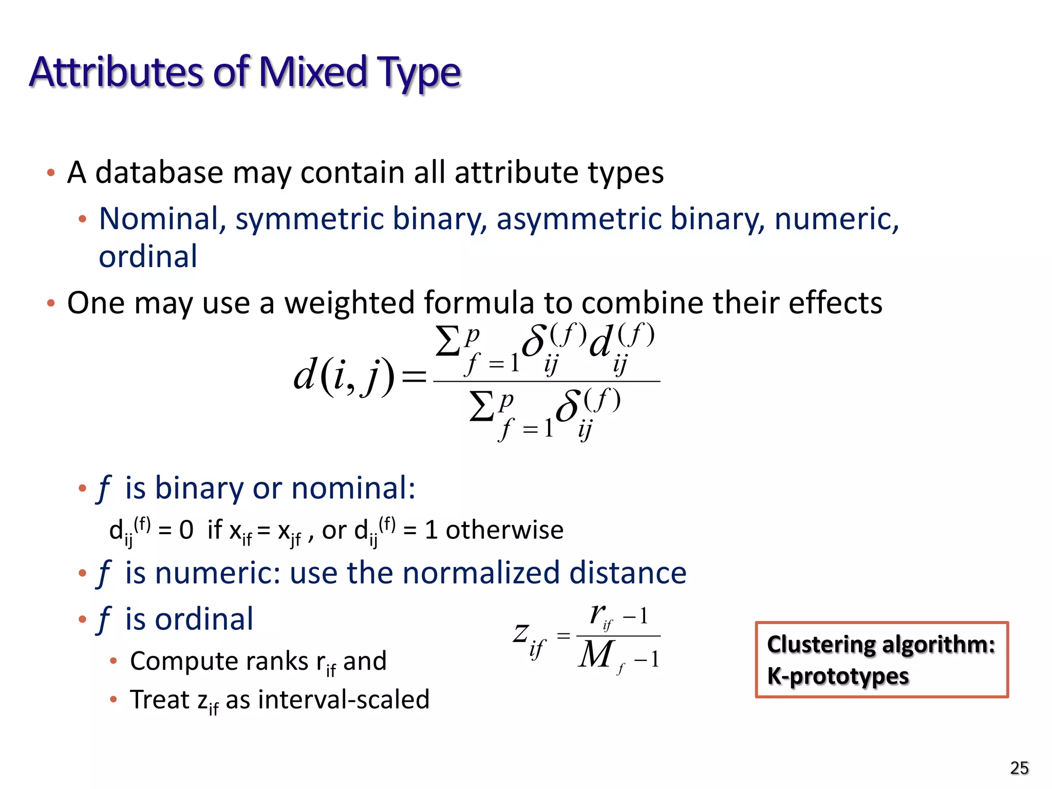
24. Ordinal Variables
• Order is important, e.g., rank
• Can be treated like interval-scaled
• replace xif by their rank
• map the range of each variable onto [0, 1] by replacing i-th object
in the f-th variable by
• compute the dissimilarity using methods for interval-scaled
variables
24
1
1
−
−
=
f
if
if M
r
z
}
,...,
1
{ f
if
M
r ∈

25. Attributes of Mixed Type
• A database may contain all attribute types
• Nominal, symmetric binary, asymmetric binary, numeric,
ordinal
• One may use a weighted formula to combine their effects
• f is binary or nominal:
dij
(f) = 0 if xif = xjf , or dij
(f) = 1 otherwise
• f is numeric: use the normalized distance
• f is ordinal
• Compute ranks rif and
• Treat zif as interval-scaled
)
(
1
)
(
)
(
1
)
,
( f
ij
p
f
f
ij
f
ij
p
f
d
j
i
d
δ
δ
=
=
Σ
Σ
=
1
1
−
−
=
f
if
M
r
zif
25
Clustering algorithm:
K-prototypes

26. Cosine Similarity
• A document can be represented by thousands of attributes, each recording the
frequency of a particular word (such as keywords) or phrase in the document.
• Other vector objects: gene features in micro-arrays, …
• Applications: information retrieval, biologic taxonomy, gene feature mapping, ...
• Cosine measure: If d1 and d2 are two vectors (e.g., term-frequency vectors), then
cos(d1, d2) = (d1 • d2) /||d1|| ||d2|| ,
where • indicates vector dot product, ||d||: the length of vector d
26
Clustering algorithm:
Spherical k-means

27. Example: Cosine Similarity
• cos(d1, d2) = (d1 • d2) /||d1|| ||d2|| ,
where • indicates vector dot product, ||d|: the length of vector d
• Ex: Find the similarity between documents 1 and 2.
d1 = (5, 0, 3, 0, 2, 0, 0, 2, 0, 0)
d2 = (3, 0, 2, 0, 1, 1, 0, 1, 0, 1)
d1•d2 = 5*3+0*0+3*2+0*0+2*1+0*1+0*1+2*1+0*0+0*1 = 25
||d1||= (5*5+0*0+3*3+0*0+2*2+0*0+0*0+2*2+0*0+0*0)0.5=(42)0.5 = 6.481
||d2||= (3*3+0*0+2*2+0*0+1*1+1*1+0*0+1*1+0*0+1*1)0.5=(17)0.5 = 4.12
cos(d1, d2 ) = 0.94
27

28. Evaluation and Other Practical Issues
•Evaluation of Clustering
•Similarity and Dissimilarity
•Summary
28

29. Summary
•Evaluation of Clustering
• Purity, NMI, RI, F-measure
•Similarity and Dissimilarity
• Nominal attributes
• Numerical attributes
• Combine attributes
• High dimensional feature vector
29