Download as PDF, PPTX
![1
Hierarchical Clustering
Class Algorithmic Methods of Data Mining
Program M. Sc. Data Science
University Sapienza University of Rome
Semester Fall 2015
Lecturer Carlos Castillo http://chato.cl/
Sources:
● Mohammed J. Zaki, Wagner Meira, Jr., Data Mining and Analysis:
Fundamental Concepts and Algorithms, Cambridge University
Press, May 2014. Chapter 14. [download]
● Evimaria Terzi: Data Mining course at Boston University
http://www.cs.bu.edu/~evimaria/cs565-13.html](https://image.slidesharecdn.com/log6kntt4i4dgwfwbpxw-signature-75c4ed0a4b22d2fef90396cdcdae85b38911f9dce0924a5c52076dfcf2a19db1-poli-151222094044/75/Hierarchical-Clustering-1-2048.jpg)
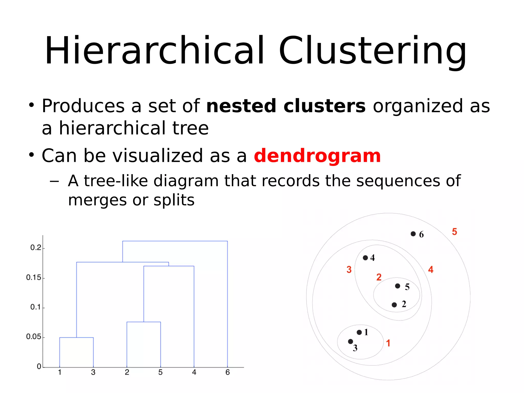
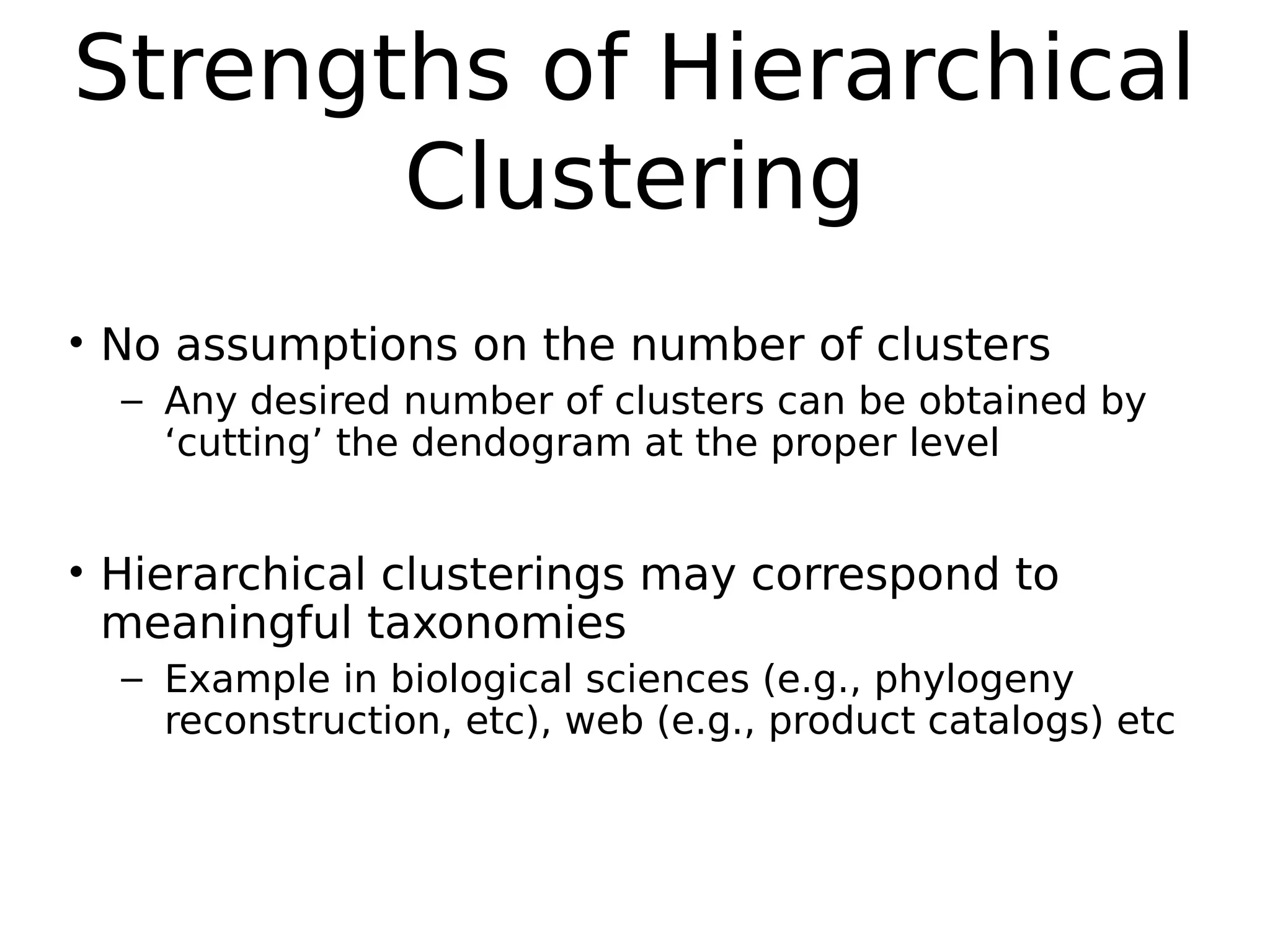
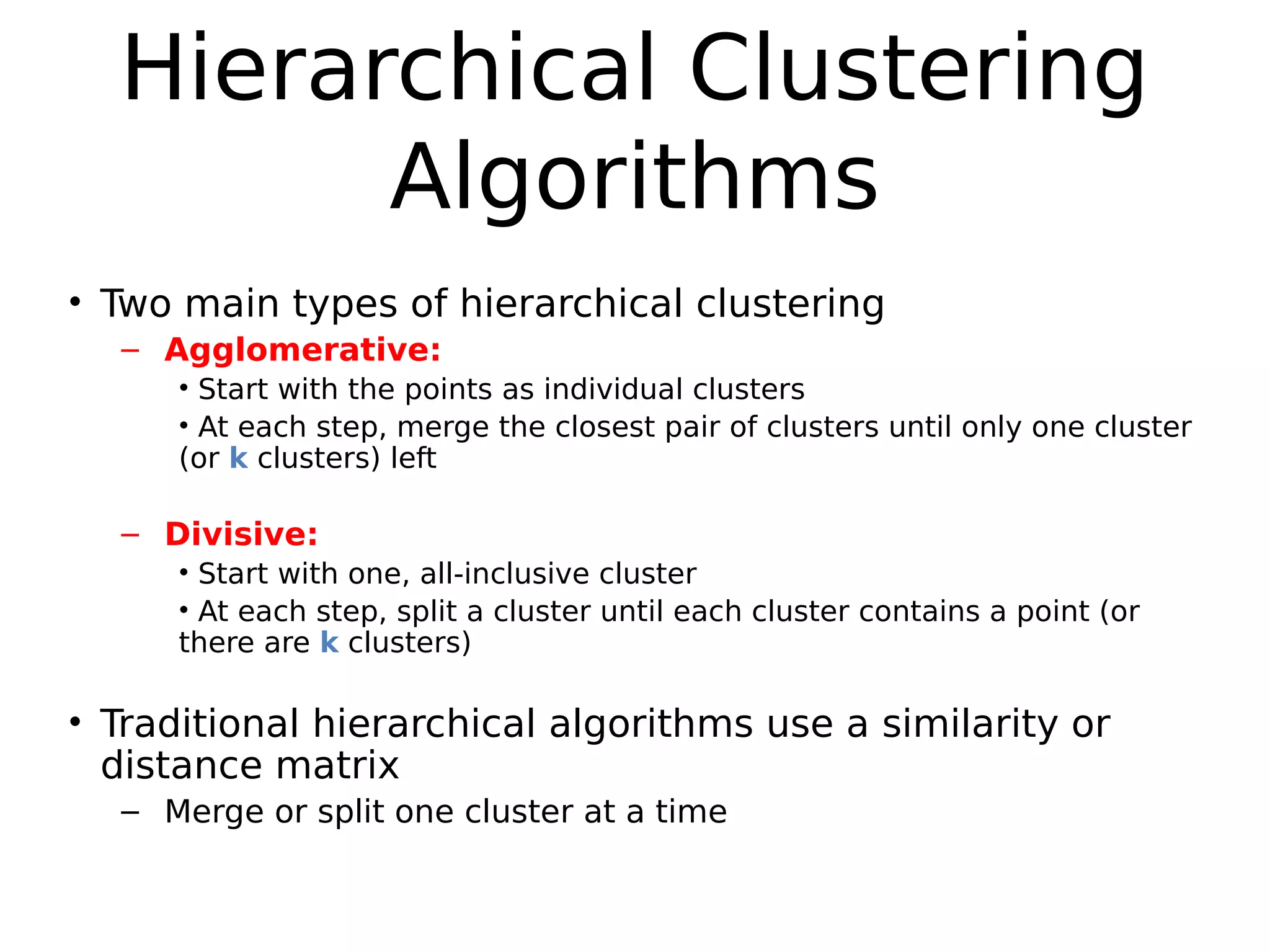
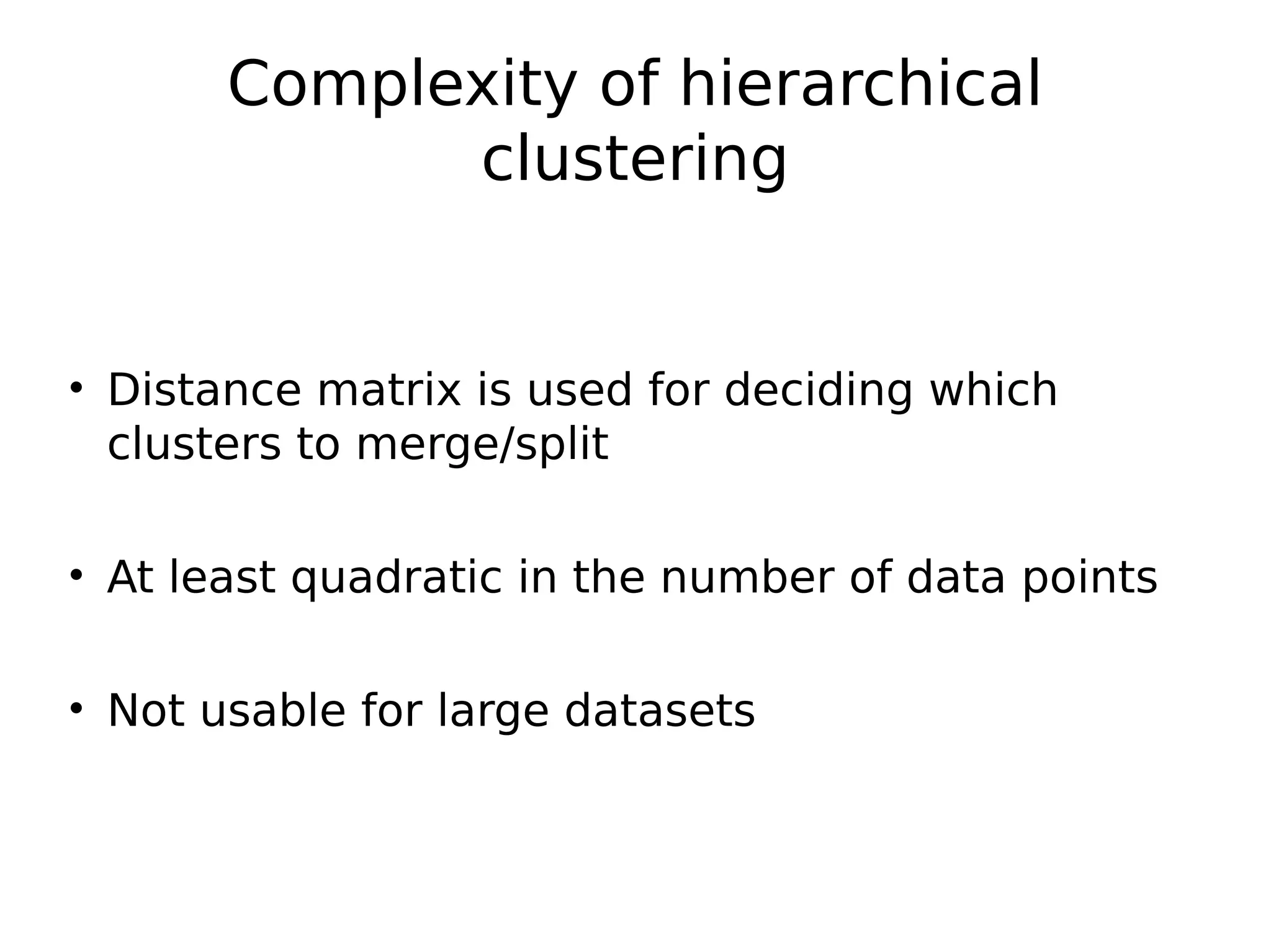
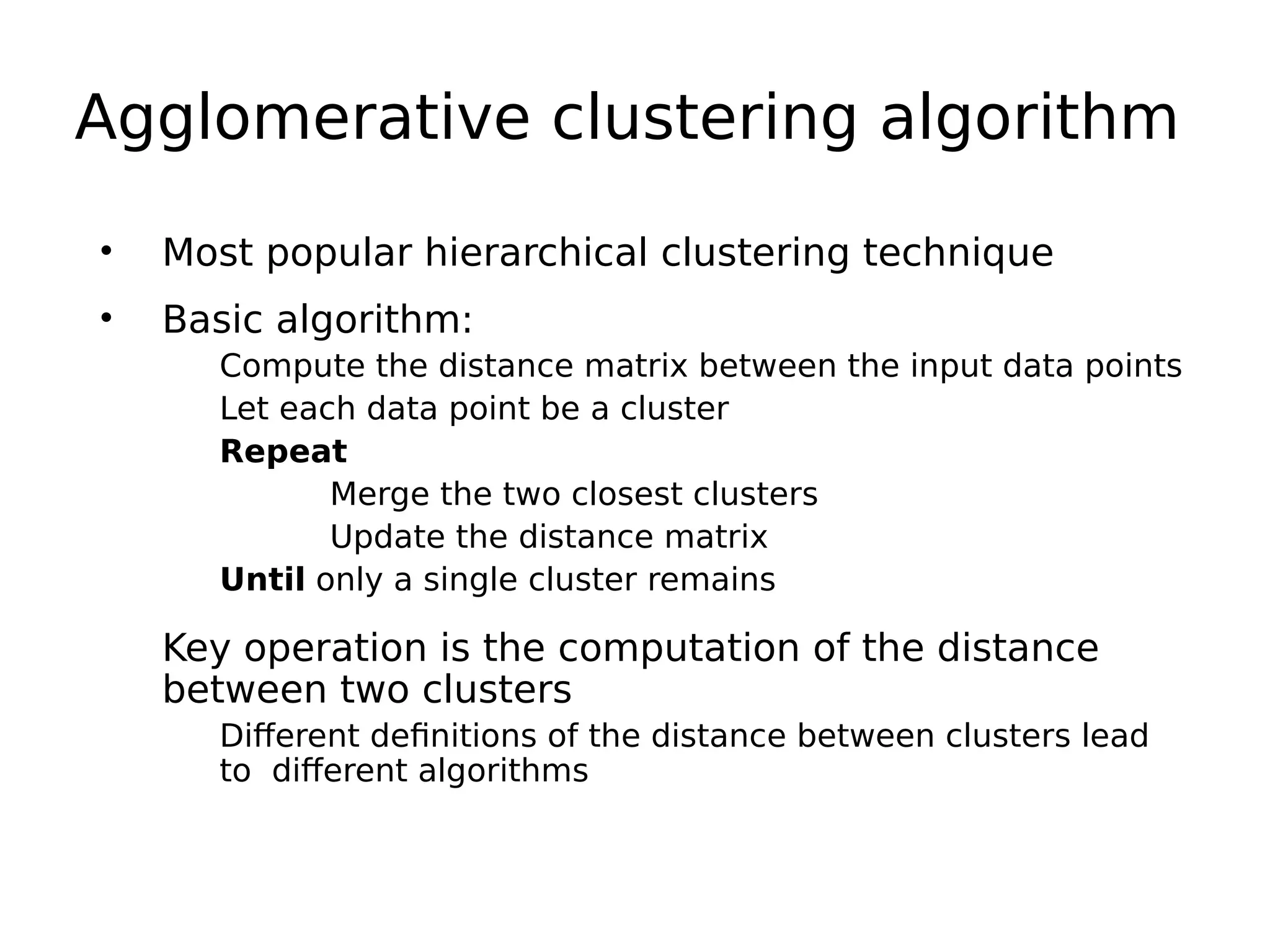
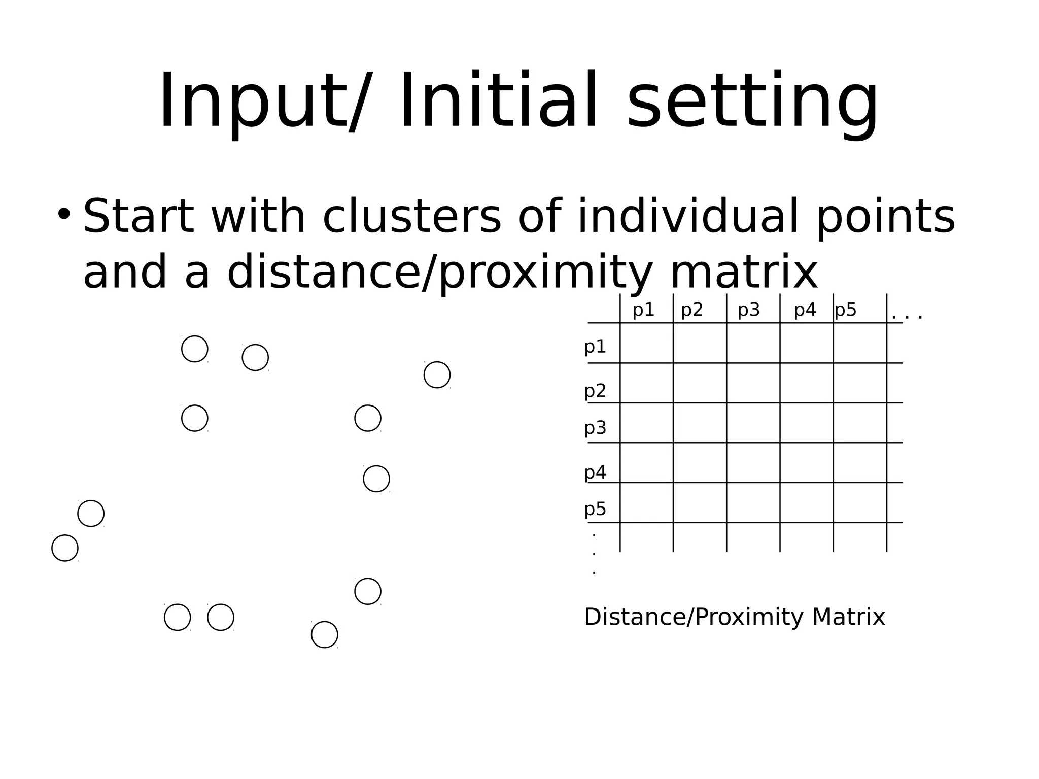
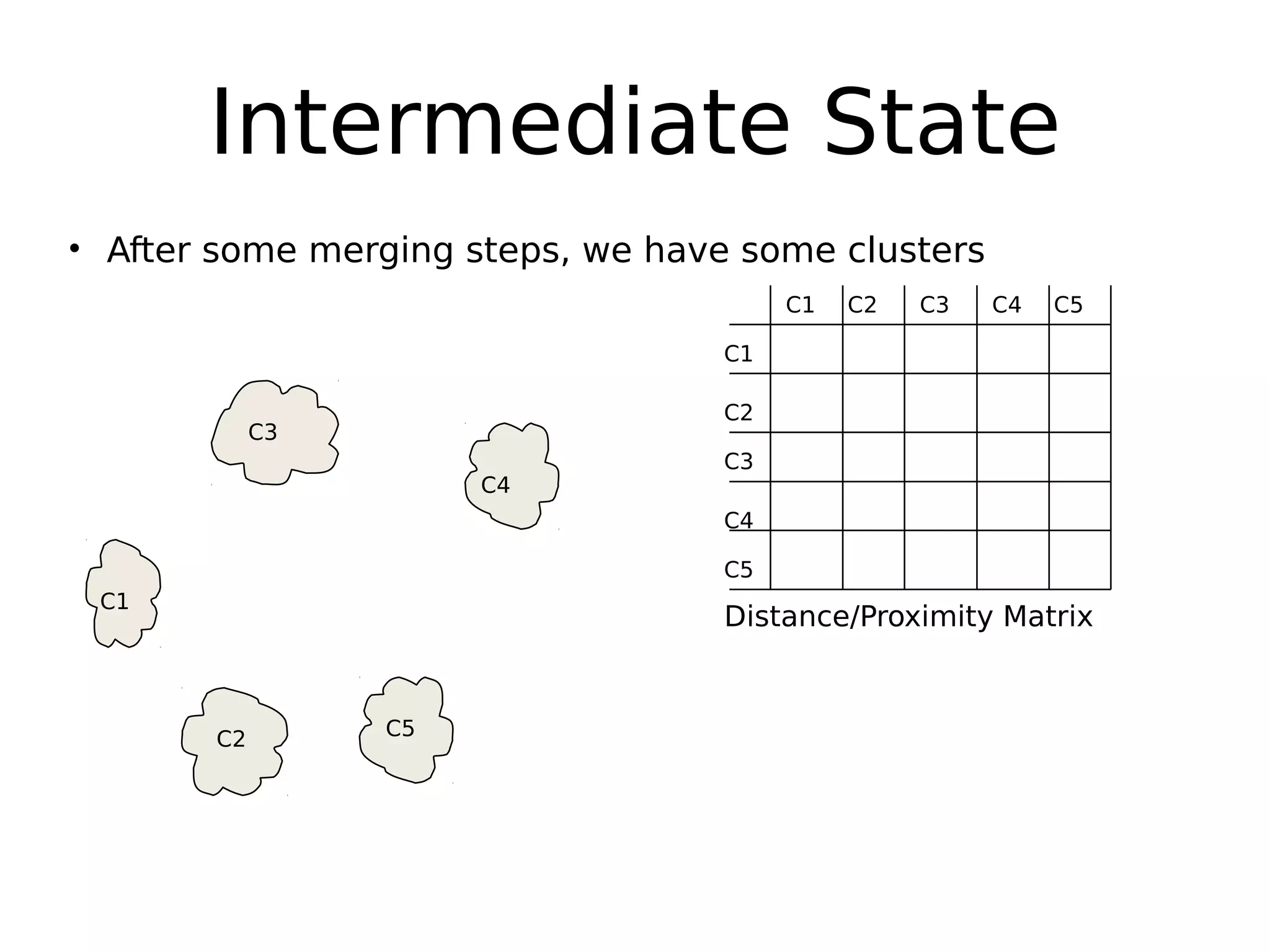
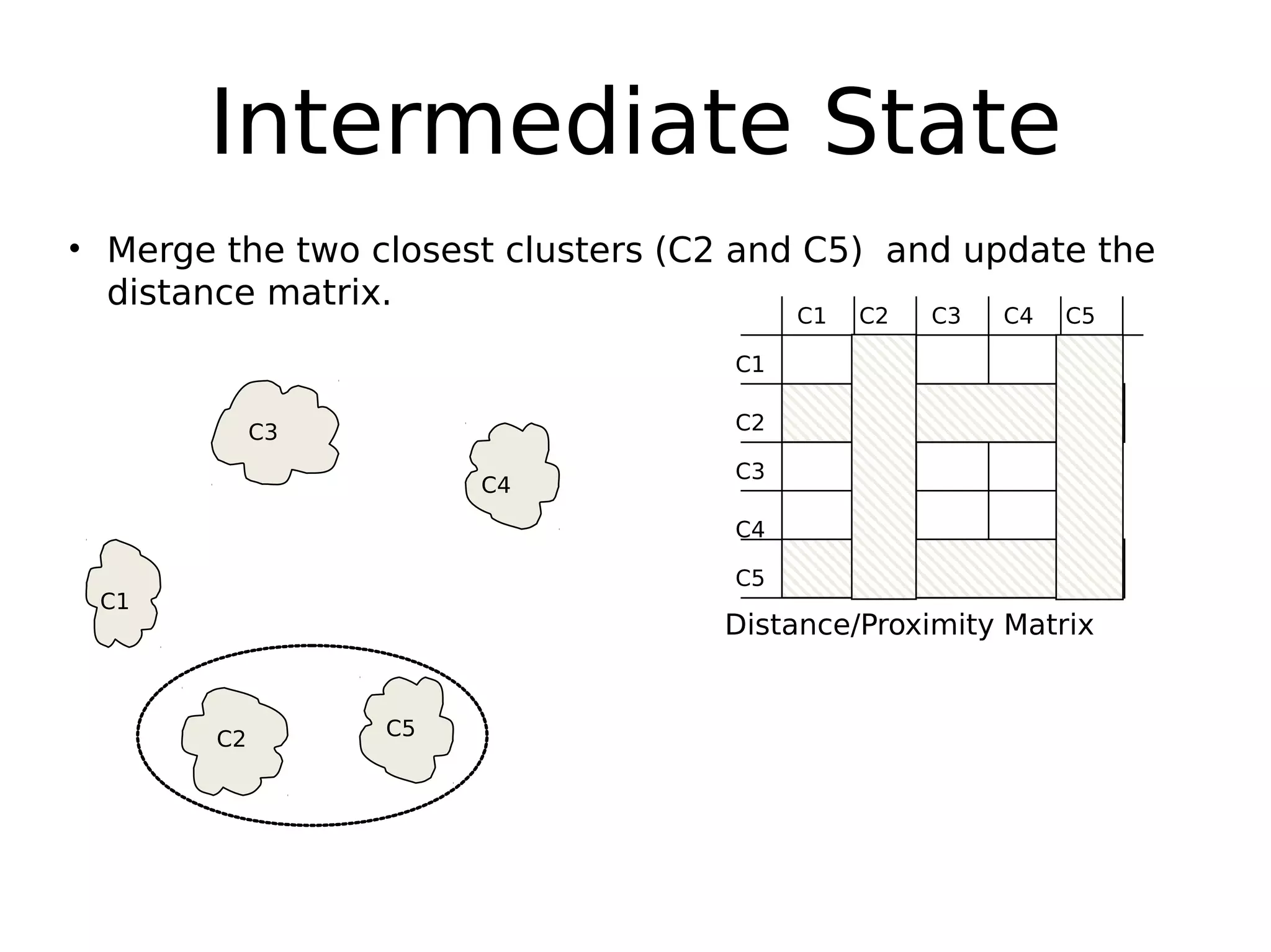
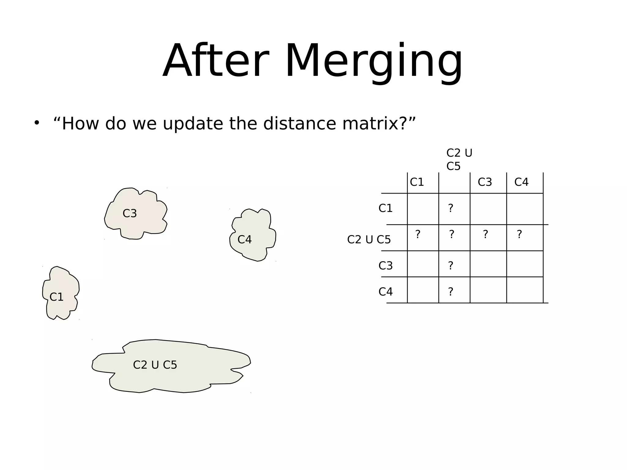
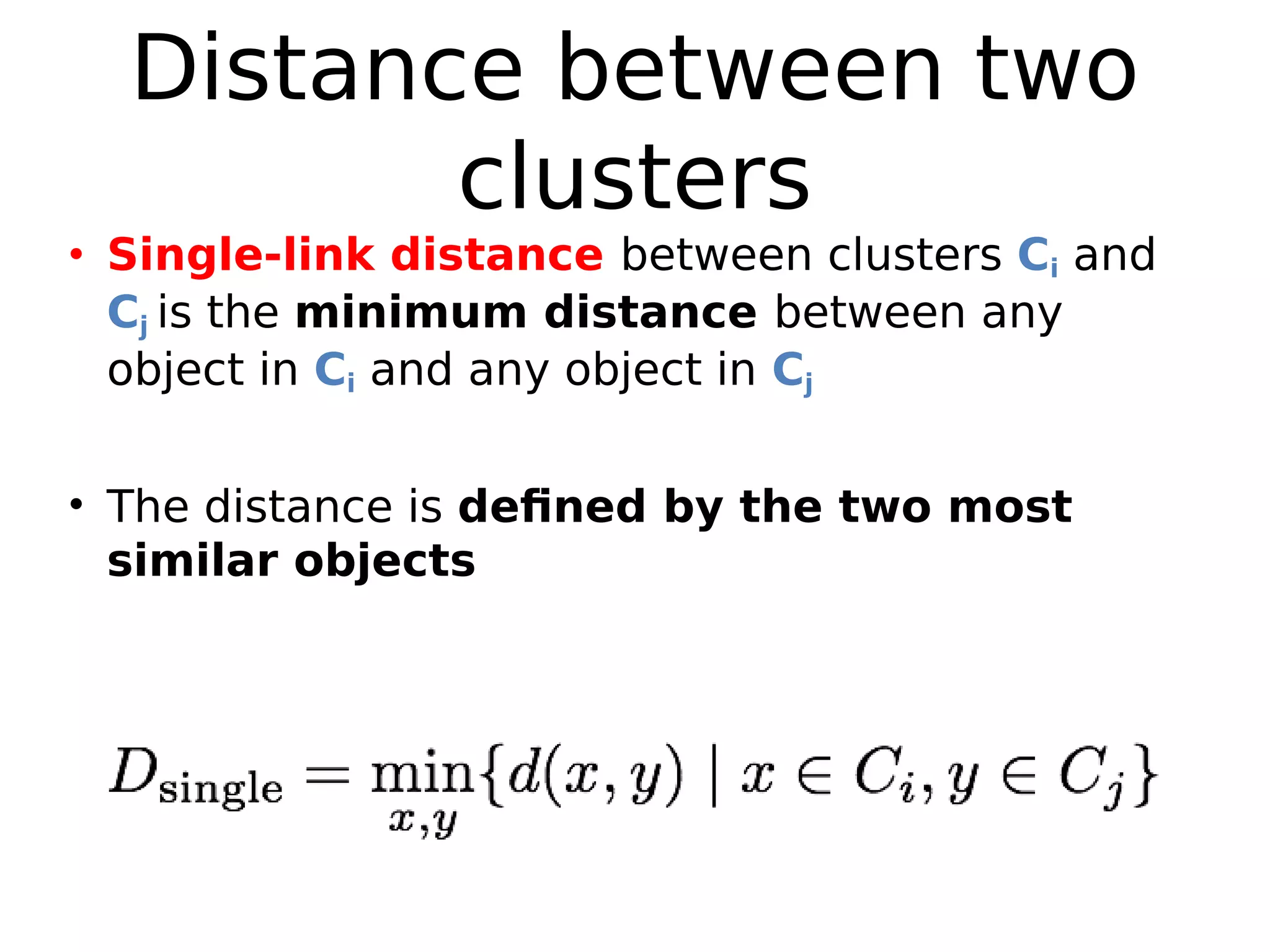
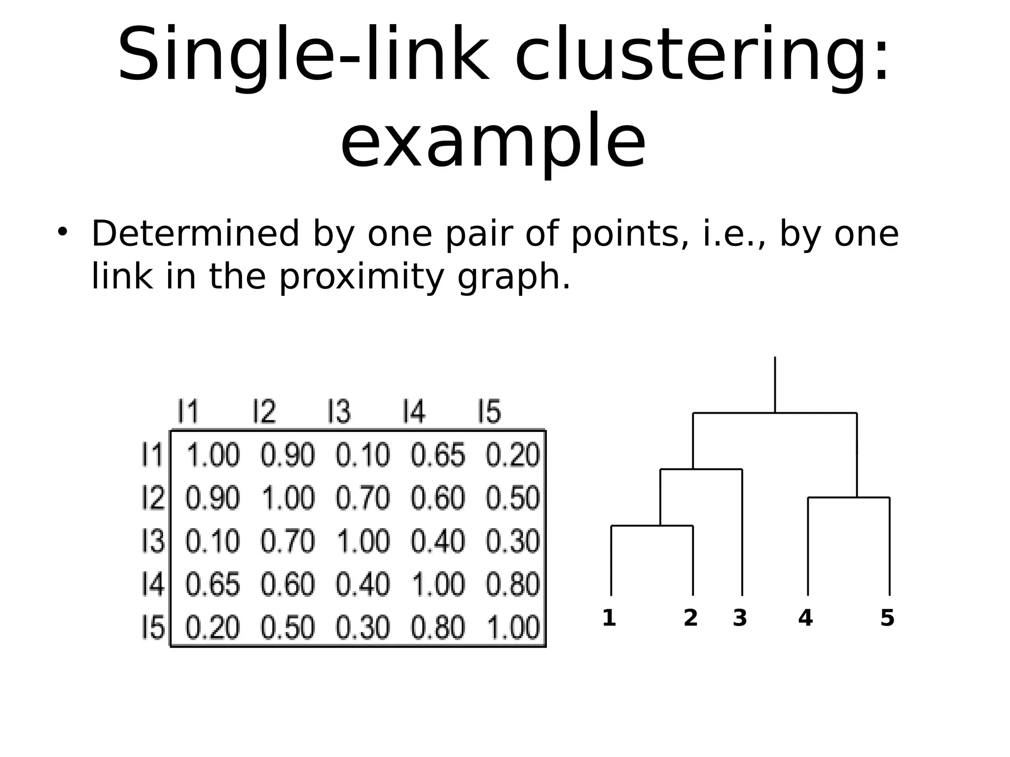
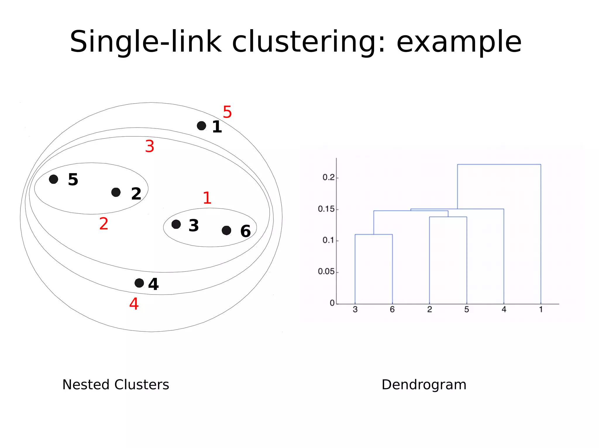
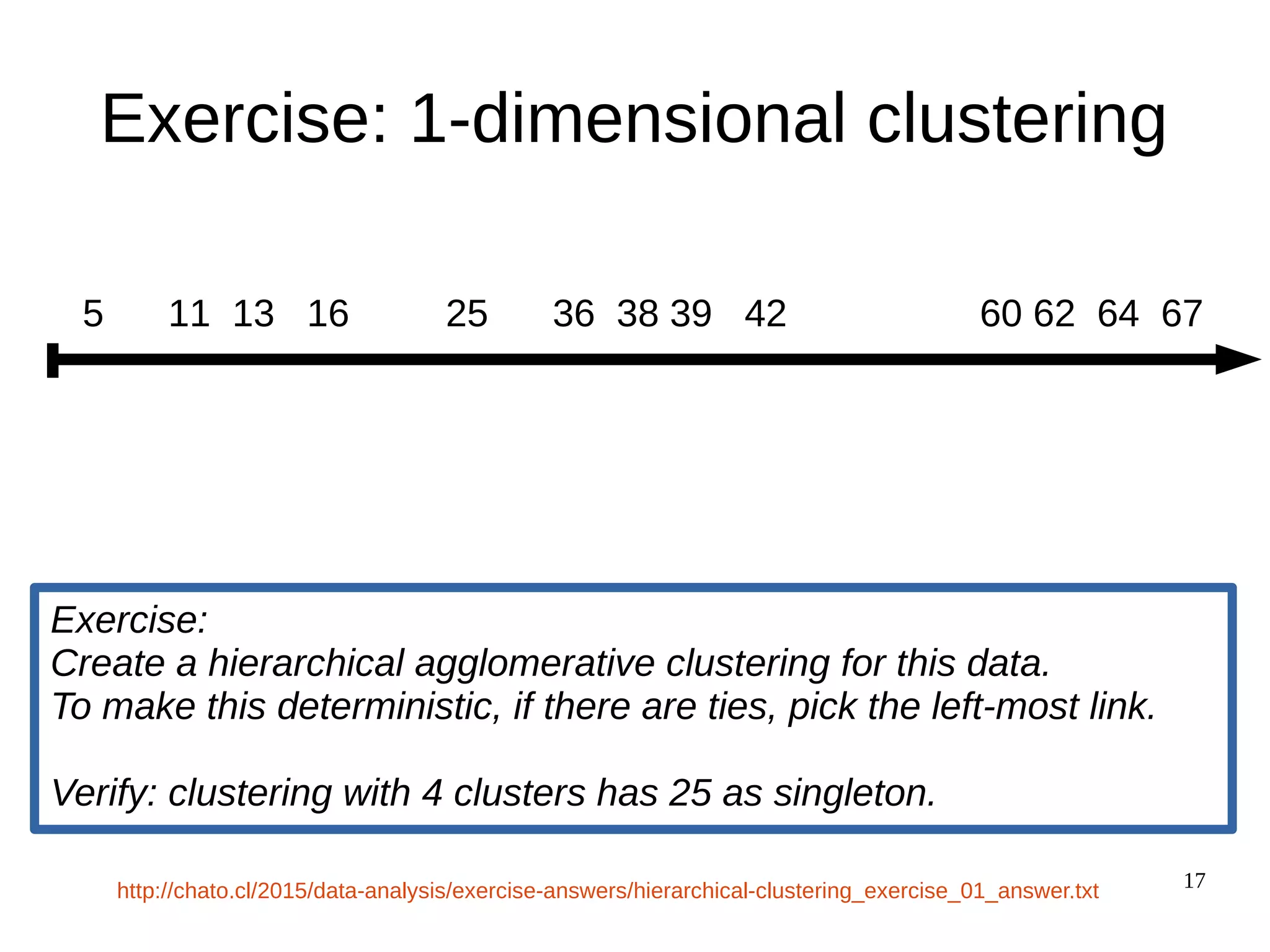
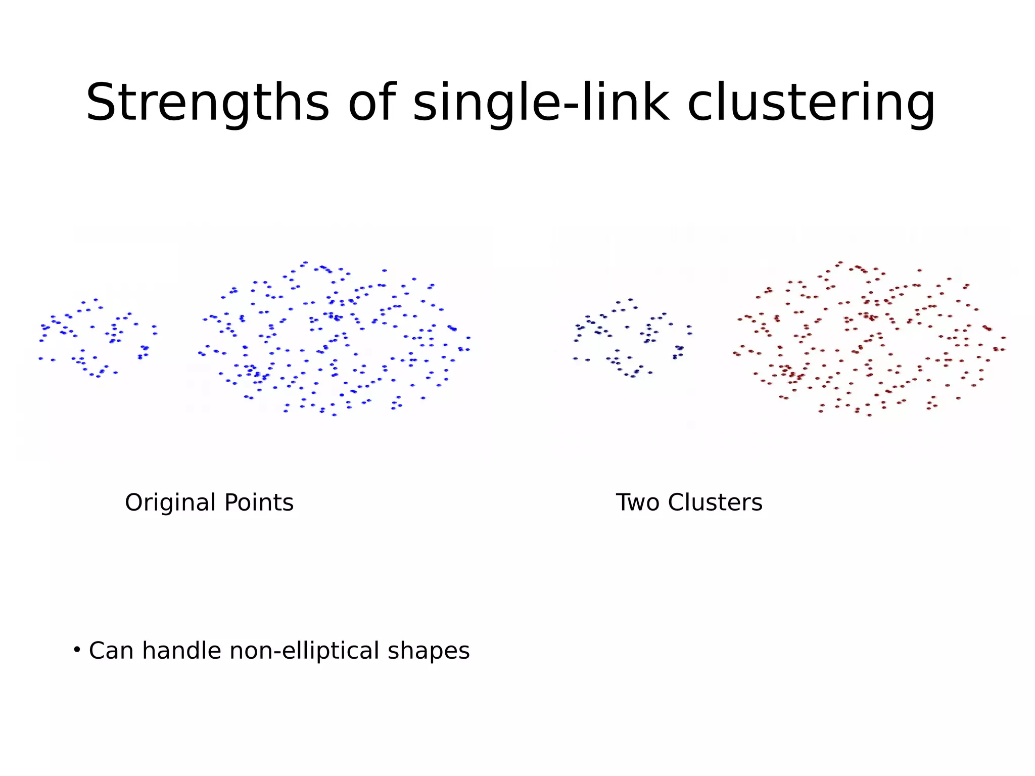
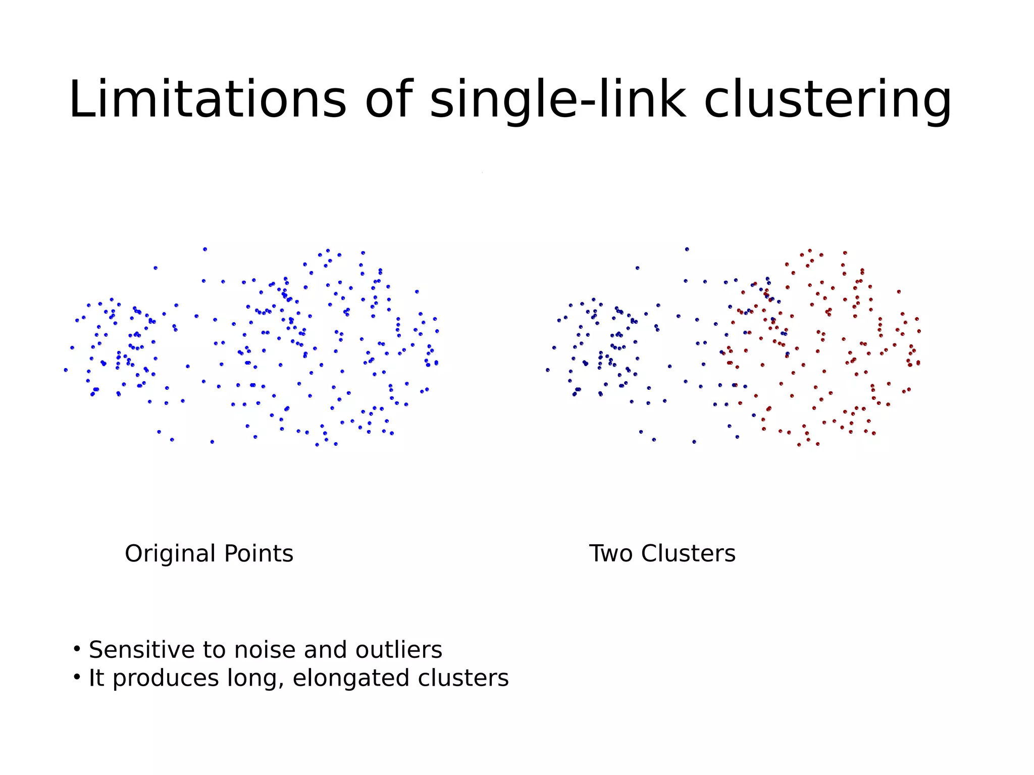
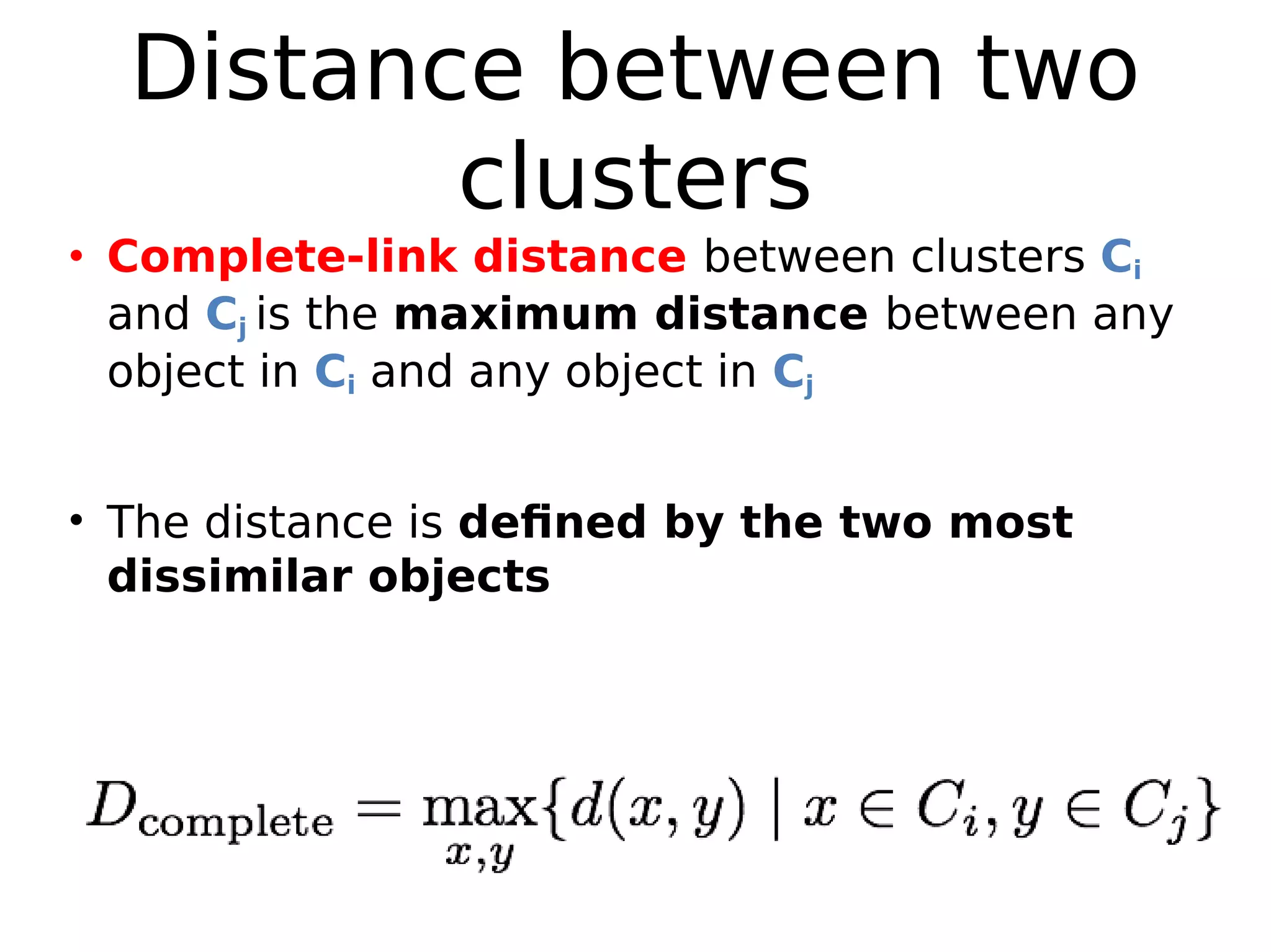
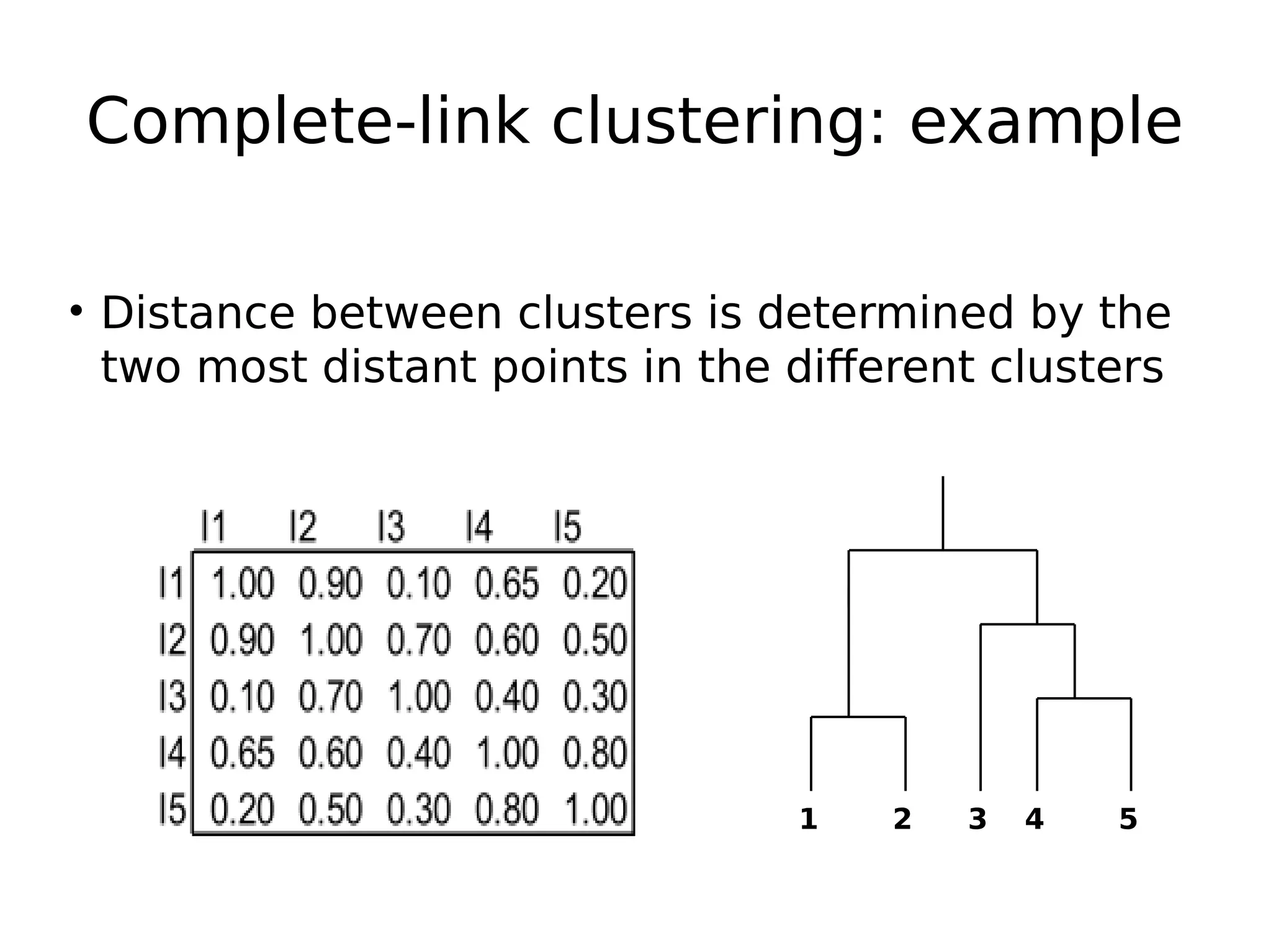
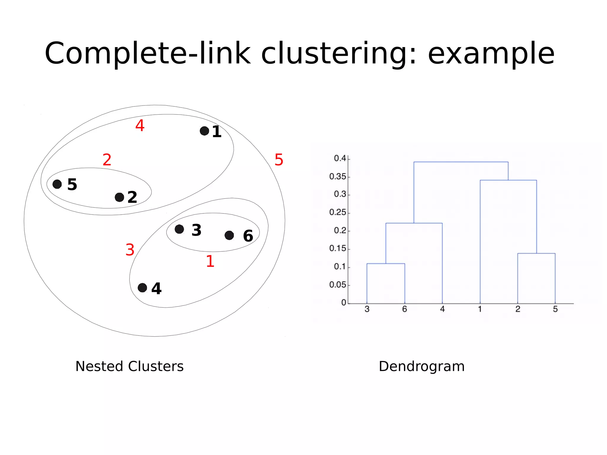
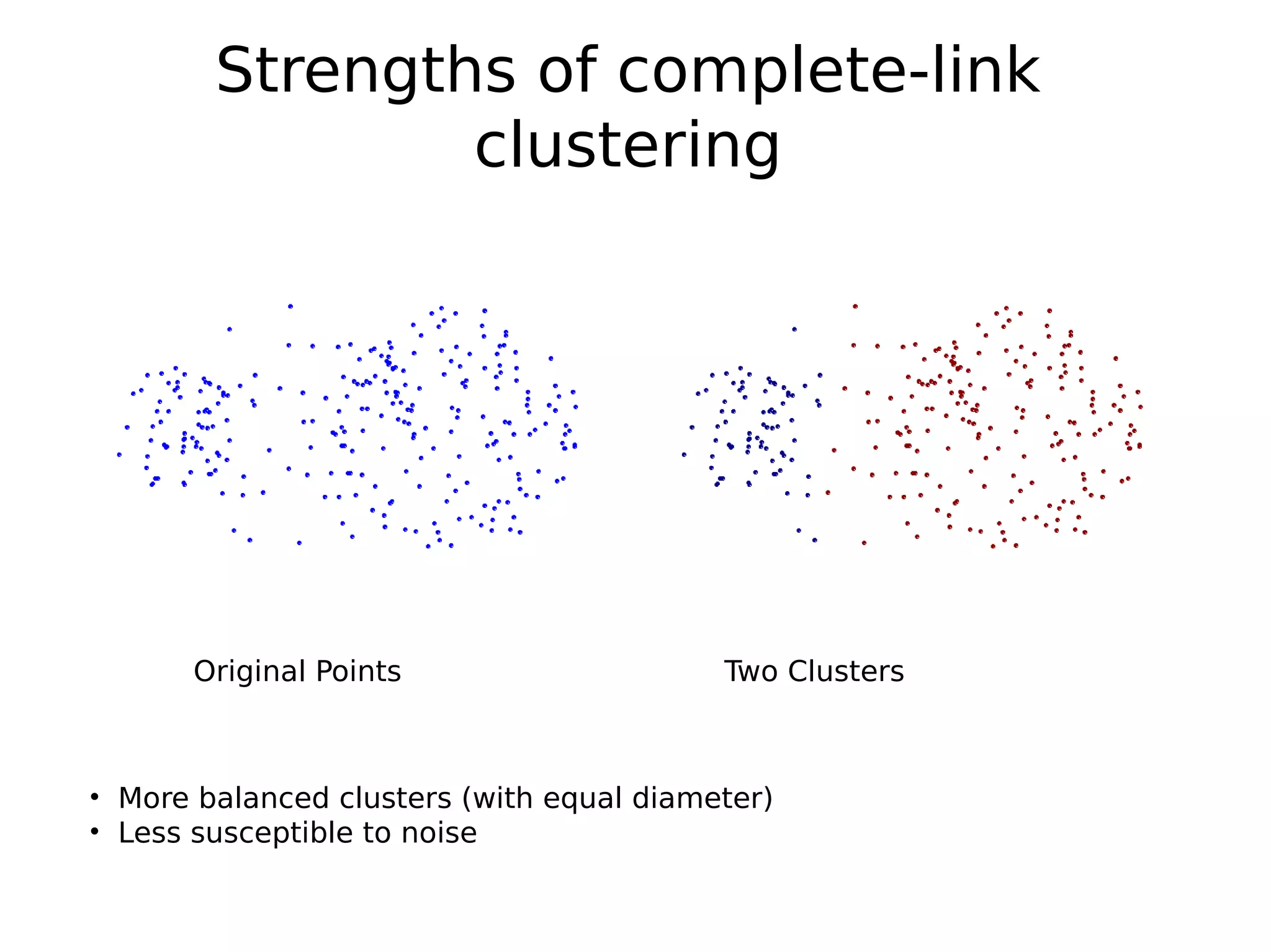
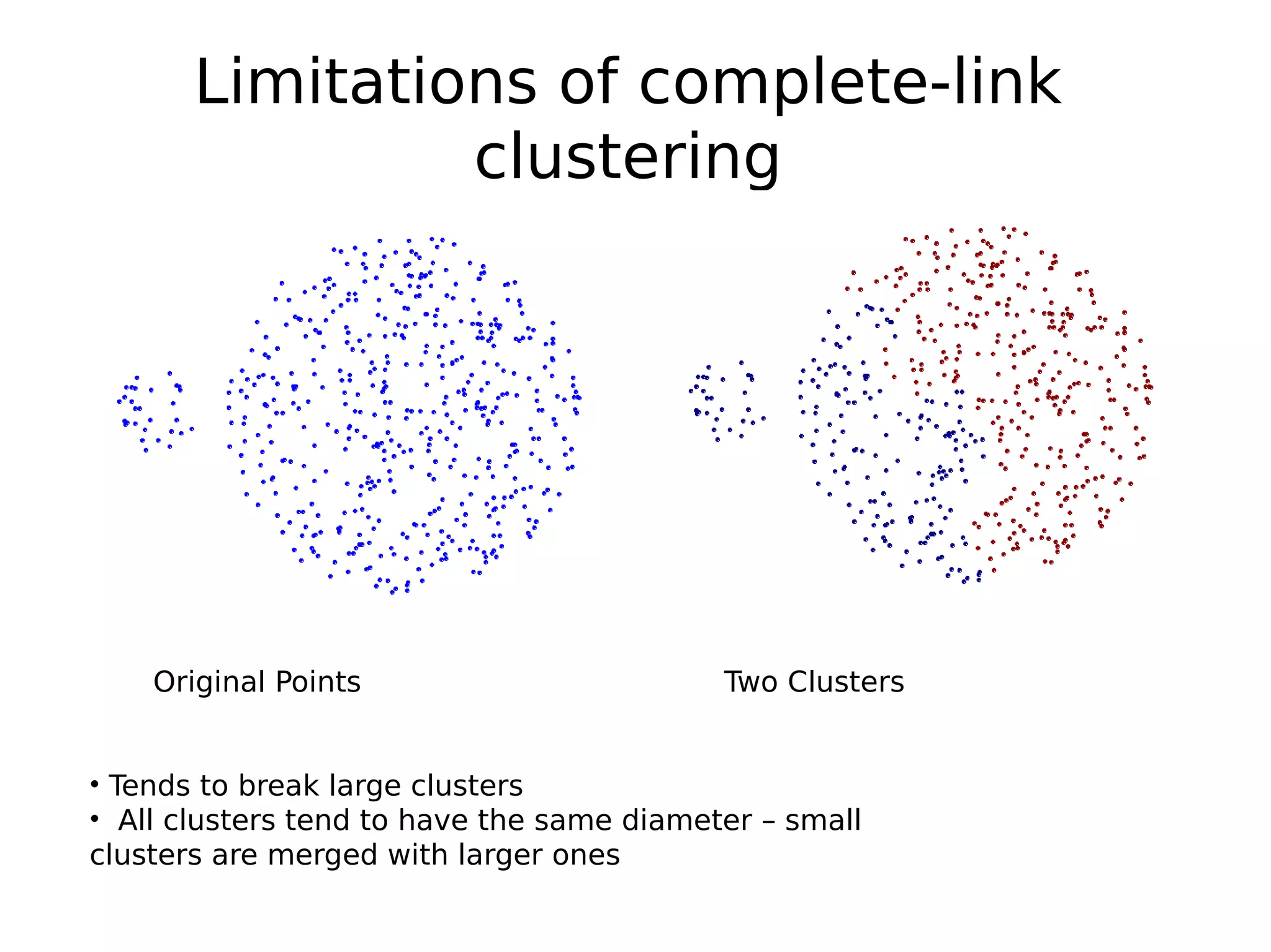
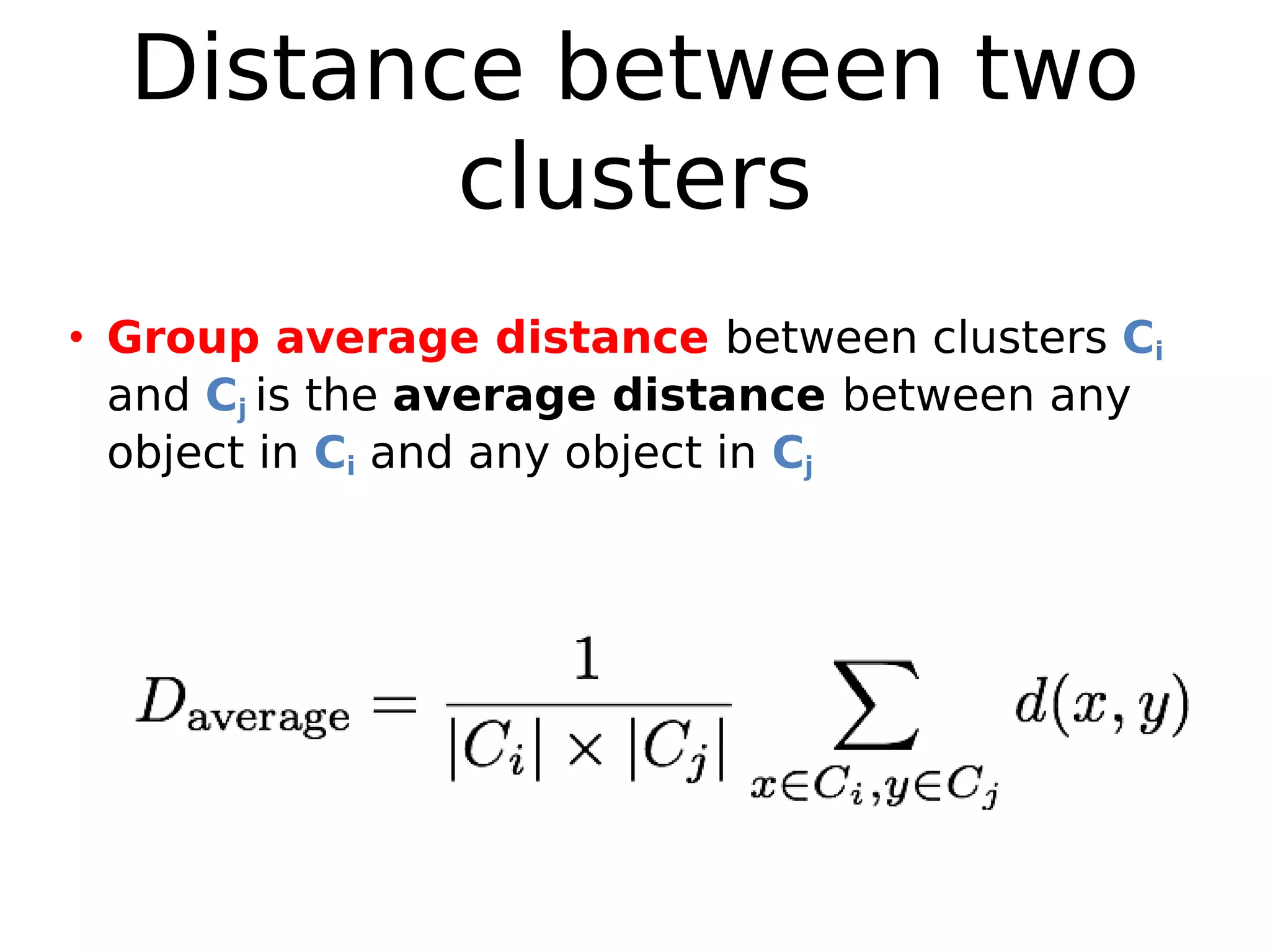
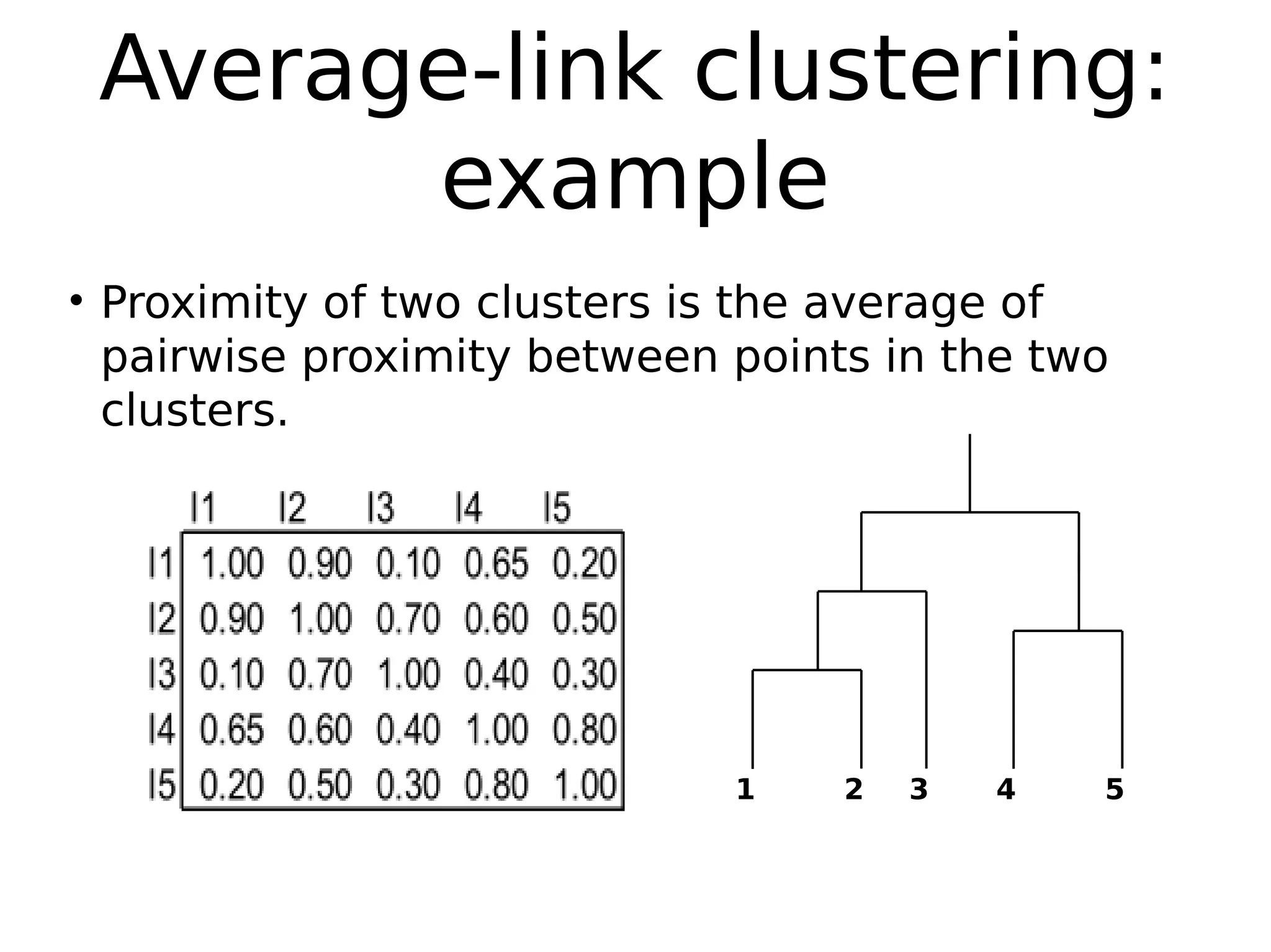
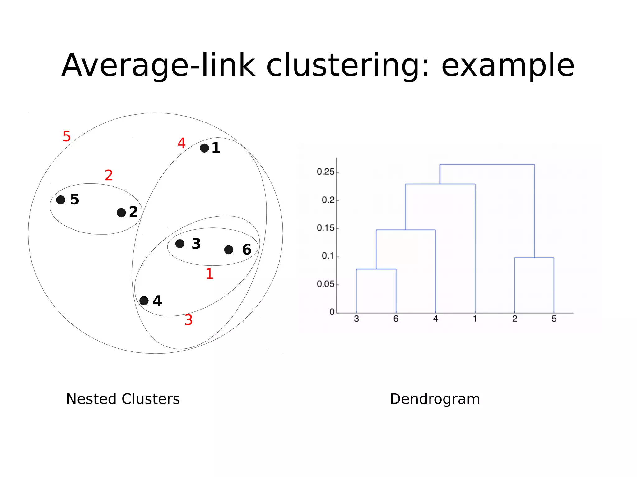
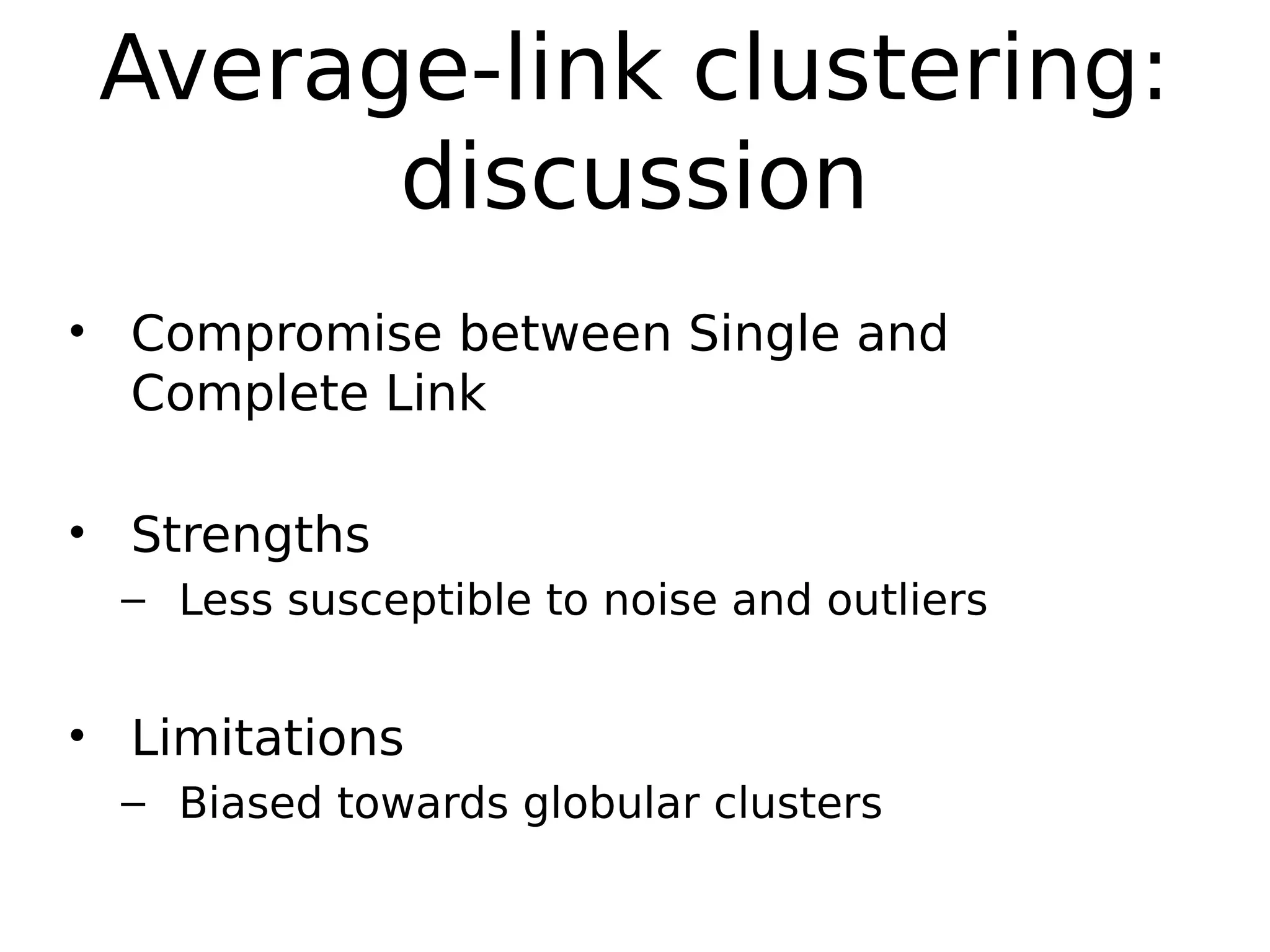
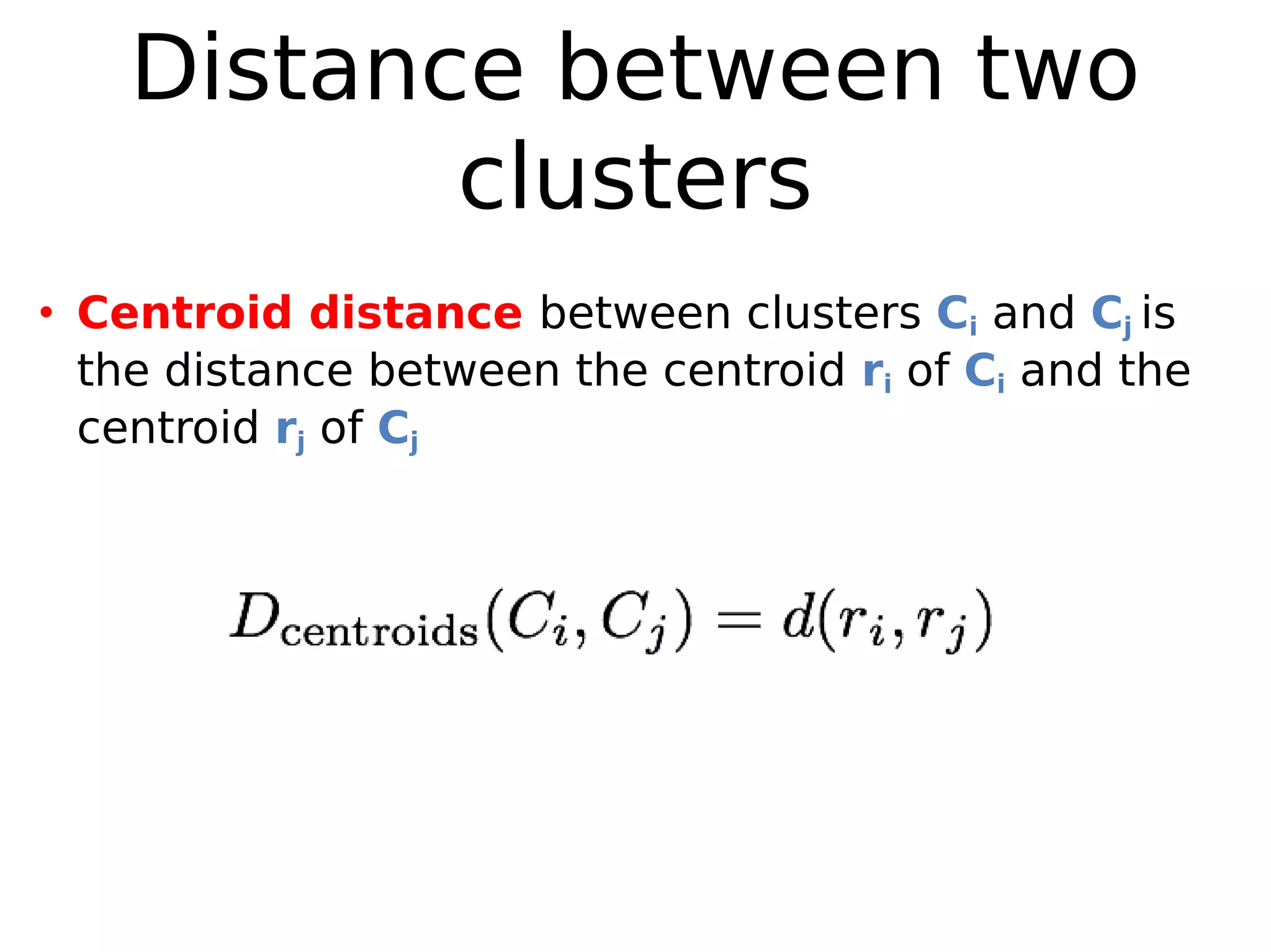
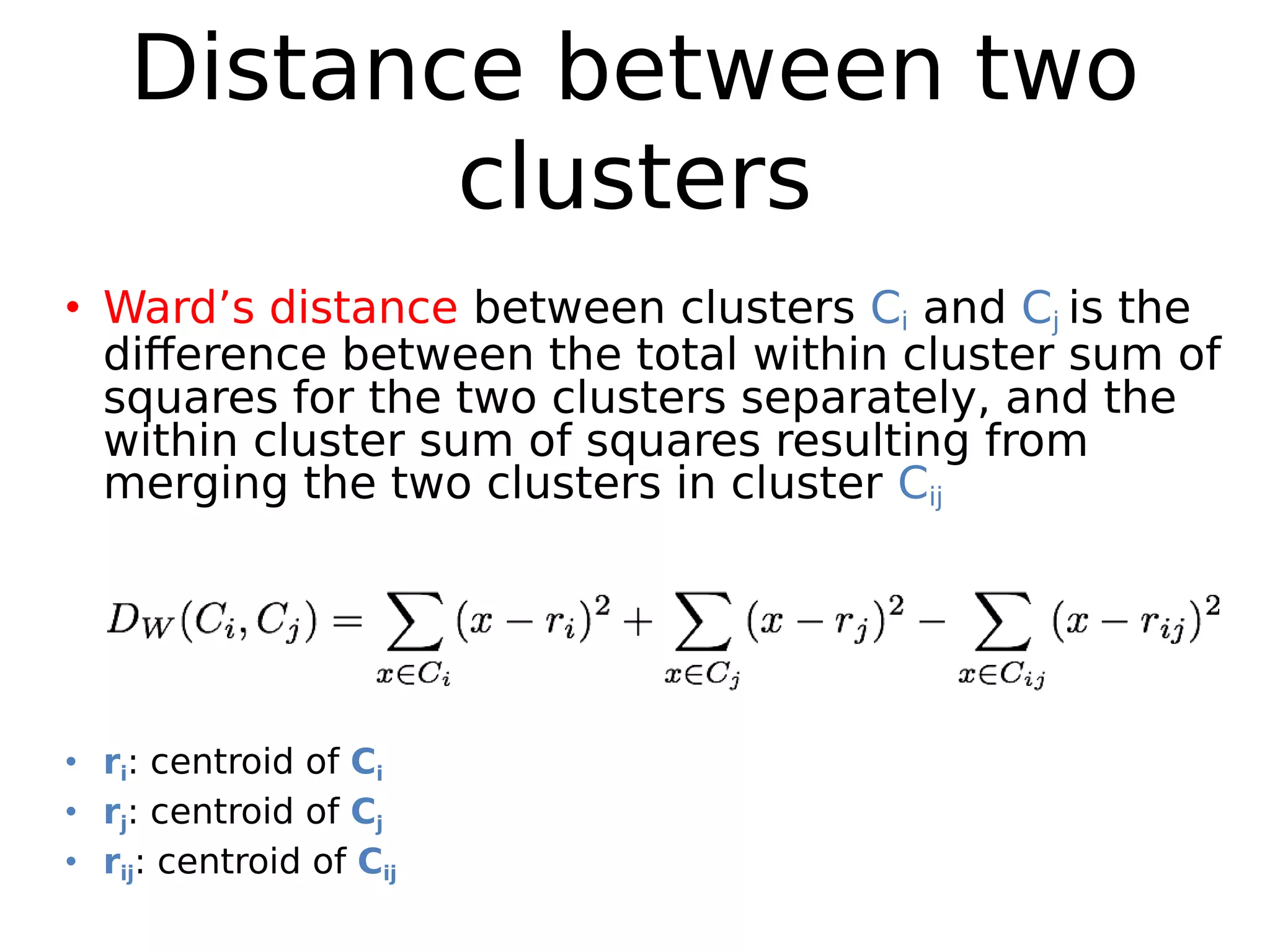
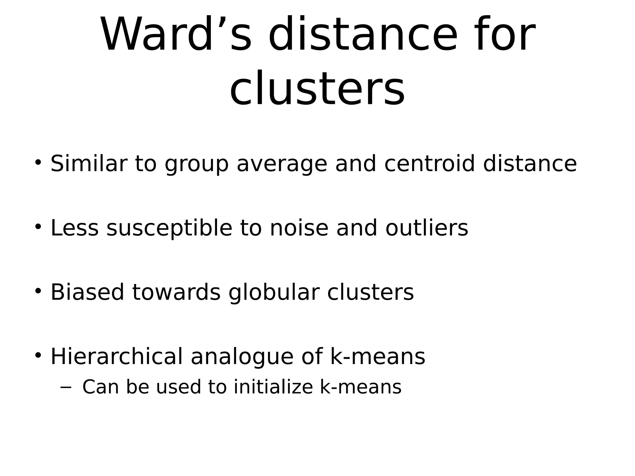
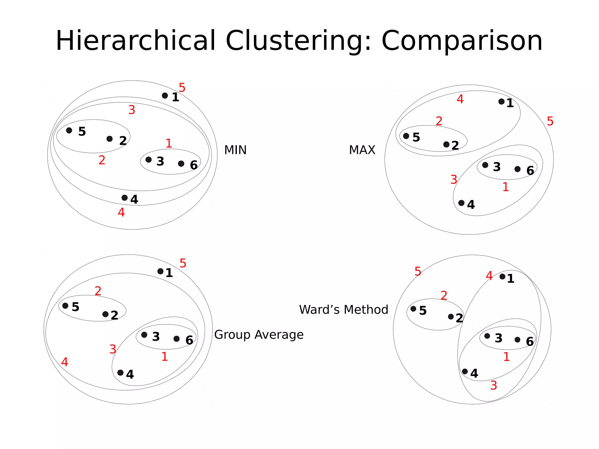
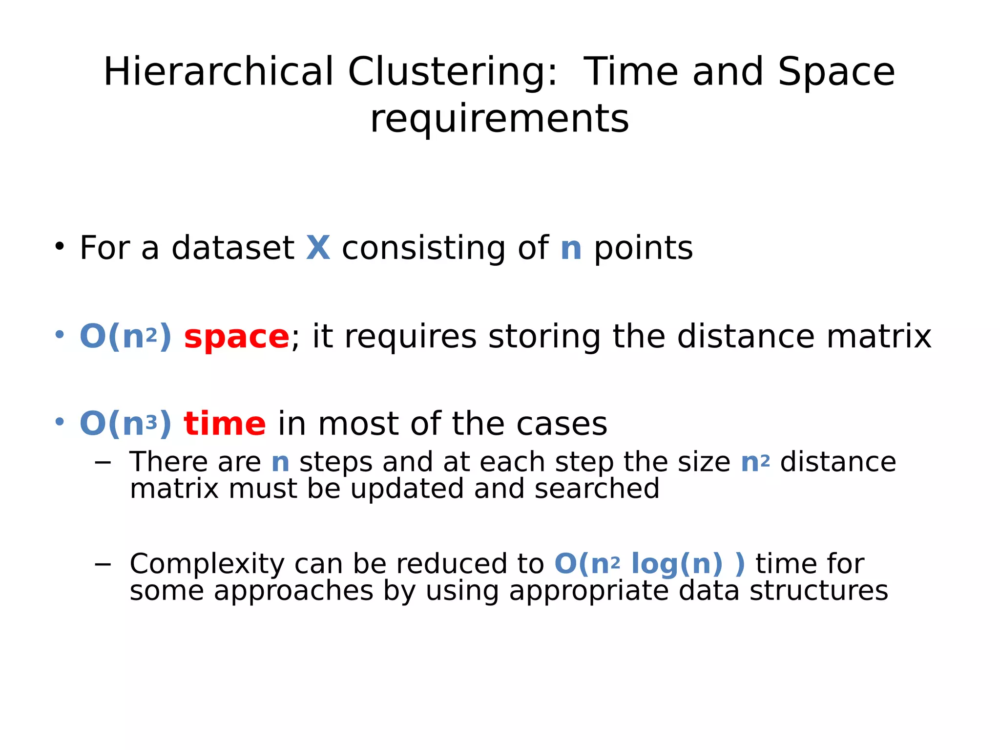

The document discusses hierarchical clustering, an algorithmic method in data mining that organizes data into nested clusters visualized as dendrograms. It elaborates on two main types of hierarchical clustering—agglomerative and divisive—detailing their processes, strengths, and limitations. Additionally, it compares different distance metrics used in clustering, such as single-link, complete-link, average-link, and Ward's method, highlighting their impacts on clustering results.


![Vibe Coding vs. Spec-Driven Development [Free Meetup]](https://cdn.slidesharecdn.com/ss_thumbnails/vibecodingvsspecdrivendevelopment-251209105622-43f455e7-thumbnail.jpg?width=640&height=640&fit=bounds)


