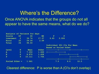
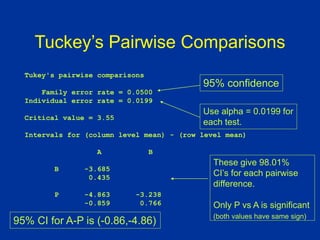
ANOVA (analysis of variance) was used to determine if the healing times of blisters (in days) were significantly different between three treatment groups: Treatment A, Treatment B, and placebo. The data met the assumptions of ANOVA. The ANOVA results showed a significant difference between the groups (p=0.006). Post hoc tests revealed the placebo group took significantly longer to heal than Treatment A, with no other significant differences between the groups.
Analysis of Variance (ANOVA) is a generalized statistical
technique used to analyze sample variances to obtain information on comparing multiple
population means.
Analysis of Variance (ANOVA) is a generalized statistical
technique used to analyze sample variances to obtain information on comparing multiple
population means.
2.0.statistical methods and determination of sample sizesalummkata1
statistical methods and determination of sample size
These guidelines focus on the validation of the bioanalytical methods generating quantitative concentration data used for pharmacokinetic and toxicokinetic parameter determinations.
These are slides I use when teaching my second year undergraduate statistics course. They are designed more for conceptual understanding, and do not have syntax for programs like SPSS or R. So it is a more conceptual and mathematical review, rather than a "how-to" computer guide.
a full lecture presentation on ANOVA .
areas covered include;
a. definition and purpose of anova
b. one-way anova
c. factorial anova
d. mutiple anova
e MANOVA
f. POST-HOC TESTS - types
f. easy step by step process of calculating post hoc test.
Please Subscribe to this Channel for more solutions and lectures
http://www.youtube.com/onlineteaching
Chapter 12: Analysis of Variance
12.1: One-Way ANOVA
06-04-2024 - NYC Tech Week - Discussion on Vector Databases, Unstructured Data and AI
Discussion on Vector Databases, Unstructured Data and AI
https://www.meetup.com/unstructured-data-meetup-new-york/
This meetup is for people working in unstructured data. Speakers will come present about related topics such as vector databases, LLMs, and managing data at scale. The intended audience of this group includes roles like machine learning engineers, data scientists, data engineers, software engineers, and PMs.This meetup was formerly Milvus Meetup, and is sponsored by Zilliz maintainers of Milvus.
06-04-2024 - NYC Tech Week - Discussion on Vector Databases, Unstructured Data and AI
Round table discussion of vector databases, unstructured data, ai, big data, real-time, robots and Milvus.
A lively discussion with NJ Gen AI Meetup Lead, Prasad and Procure.FYI's Co-Found
Show drafts
volume_up
Empowering the Data Analytics Ecosystem: A Laser Focus on Value
The data analytics ecosystem thrives when every component functions at its peak, unlocking the true potential of data. Here's a laser focus on key areas for an empowered ecosystem:
1. Democratize Access, Not Data:
Granular Access Controls: Provide users with self-service tools tailored to their specific needs, preventing data overload and misuse.
Data Catalogs: Implement robust data catalogs for easy discovery and understanding of available data sources.
2. Foster Collaboration with Clear Roles:
Data Mesh Architecture: Break down data silos by creating a distributed data ownership model with clear ownership and responsibilities.
Collaborative Workspaces: Utilize interactive platforms where data scientists, analysts, and domain experts can work seamlessly together.
3. Leverage Advanced Analytics Strategically:
AI-powered Automation: Automate repetitive tasks like data cleaning and feature engineering, freeing up data talent for higher-level analysis.
Right-Tool Selection: Strategically choose the most effective advanced analytics techniques (e.g., AI, ML) based on specific business problems.
4. Prioritize Data Quality with Automation:
Automated Data Validation: Implement automated data quality checks to identify and rectify errors at the source, minimizing downstream issues.
Data Lineage Tracking: Track the flow of data throughout the ecosystem, ensuring transparency and facilitating root cause analysis for errors.
5. Cultivate a Data-Driven Mindset:
Metrics-Driven Performance Management: Align KPIs and performance metrics with data-driven insights to ensure actionable decision making.
Data Storytelling Workshops: Equip stakeholders with the skills to translate complex data findings into compelling narratives that drive action.
Benefits of a Precise Ecosystem:
Sharpened Focus: Precise access and clear roles ensure everyone works with the most relevant data, maximizing efficiency.
Actionable Insights: Strategic analytics and automated quality checks lead to more reliable and actionable data insights.
Continuous Improvement: Data-driven performance management fosters a culture of learning and continuous improvement.
Sustainable Growth: Empowered by data, organizations can make informed decisions to drive sustainable growth and innovation.
By focusing on these precise actions, organizations can create an empowered data analytics ecosystem that delivers real value by driving data-driven decisions and maximizing the return on their data investment.
Levelwise PageRank with Loop-Based Dead End Handling Strategy : SHORT REPORT ...Subhajit Sahu
Abstract — Levelwise PageRank is an alternative method of PageRank computation which decomposes the input graph into a directed acyclic block-graph of strongly connected components, and processes them in topological order, one level at a time. This enables calculation for ranks in a distributed fashion without per-iteration communication, unlike the standard method where all vertices are processed in each iteration. It however comes with a precondition of the absence of dead ends in the input graph. Here, the native non-distributed performance of Levelwise PageRank was compared against Monolithic PageRank on a CPU as well as a GPU. To ensure a fair comparison, Monolithic PageRank was also performed on a graph where vertices were split by components. Results indicate that Levelwise PageRank is about as fast as Monolithic PageRank on the CPU, but quite a bit slower on the GPU. Slowdown on the GPU is likely caused by a large submission of small workloads, and expected to be non-issue when the computation is performed on massive graphs.
Opendatabay - Open Data Marketplace.pptxOpendatabay
Opendatabay.com unlocks the power of data for everyone. Open Data Marketplace fosters a collaborative hub for data enthusiasts to explore, share, and contribute to a vast collection of datasets.
First ever open hub for data enthusiasts to collaborate and innovate. A platform to explore, share, and contribute to a vast collection of datasets. Through robust quality control and innovative technologies like blockchain verification, opendatabay ensures the authenticity and reliability of datasets, empowering users to make data-driven decisions with confidence. Leverage cutting-edge AI technologies to enhance the data exploration, analysis, and discovery experience.
From intelligent search and recommendations to automated data productisation and quotation, Opendatabay AI-driven features streamline the data workflow. Finding the data you need shouldn't be a complex. Opendatabay simplifies the data acquisition process with an intuitive interface and robust search tools. Effortlessly explore, discover, and access the data you need, allowing you to focus on extracting valuable insights. Opendatabay breaks new ground with a dedicated, AI-generated, synthetic datasets.
Leverage these privacy-preserving datasets for training and testing AI models without compromising sensitive information. Opendatabay prioritizes transparency by providing detailed metadata, provenance information, and usage guidelines for each dataset, ensuring users have a comprehensive understanding of the data they're working with. By leveraging a powerful combination of distributed ledger technology and rigorous third-party audits Opendatabay ensures the authenticity and reliability of every dataset. Security is at the core of Opendatabay. Marketplace implements stringent security measures, including encryption, access controls, and regular vulnerability assessments, to safeguard your data and protect your privacy.
2. The basic ANOVA situation
Two variables: 1 Categorical, 1 Quantitative
Main Question: Do the (means of) the quantitative
variables depend on which group (given by
categorical variable) the individual is in?
If categorical variable has only 2 values:
• 2-sample t-test
ANOVA allows for 3 or more groups
3. An example ANOVA situation
Subjects: 25 patients with blisters
Treatments: Treatment A, Treatment B, Placebo
Measurement: # of days until blisters heal
Data [and means]:
• A: 5,6,6,7,7,8,9,10 [7.25]
• B: 7,7,8,9,9,10,10,11 [8.875]
• P: 7,9,9,10,10,10,11,12,13 [10.11]
Are these differences significant?
4. Informal Investigation
Graphical investigation:
• side-by-side box plots
• multiple histograms
Whether the differences between the groups are
significant depends on
• the difference in the means
• the standard deviations of each group
• the sample sizes
ANOVA determines P-value from the F statistic
5. Side by Side Boxplots
P
B
A
13
12
11
10
9
8
7
6
5
treatment
days
6. What does ANOVA do?
At its simplest (there are extensions) ANOVA
tests the following hypotheses:
H0: The means of all the groups are equal.
Ha: Not all the means are equal
• doesn’t say how or which ones differ.
• Can follow up with “multiple comparisons”
Note: we usually refer to the sub-populations as
“groups” when doing ANOVA.
7. Assumptions of ANOVA
• each group is approximately normal
check this by looking at histograms and/or
normal quantile plots, or use assumptions
can handle some nonnormality, but not
severe outliers
• standard deviations of each group are
approximately equal
rule of thumb: ratio of largest to smallest
sample st. dev. must be less than 2:1
8. Normality Check
We should check for normality using:
• assumptions about population
• histograms for each group
• normal quantile plot for each group
With such small data sets, there really isn’t a
really good way to check normality from data,
but we make the common assumption that
physical measurements of people tend to be
normally distributed.
9. Standard Deviation Check
Compare largest and smallest standard deviations:
• largest: 1.764
• smallest: 1.458
• 1.458 x 2 = 2.916 > 1.764
Note: variance ratio of 4:1 is equivalent.
Variable treatment N Mean Median StDev
days A 8 7.250 7.000 1.669
B 8 8.875 9.000 1.458
P 9 10.111 10.000 1.764
10. Notation for ANOVA
• n = number of individuals all together
• I = number of groups
• = mean for entire data set is
Group i has
• ni = # of individuals in group i
• xij = value for individual j in group i
• = mean for group i
• si = standard deviation for group i
i
x
x
11. How ANOVA works (outline)
ANOVA measures two sources of variation in the data and
compares their relative sizes
• variation BETWEEN groups
• for each data value look at the difference between
its group mean and the overall mean
• variation WITHIN groups
• for each data value we look at the difference
between that value and the mean of its group
2
i
ij x
x
2
x
xi
12. The ANOVA F-statistic is a ratio of the
Between Group Variaton divided by the
Within Group Variation:
MSE
MSG
Within
Between
F
A large F is evidence against H0, since it
indicates that there is more difference
between groups than within groups.
13. Minitab ANOVA Output
Analysis of Variance for days
Source DF SS MS F P
treatment 2 34.74 17.37 6.45 0.006
Error 22 59.26 2.69
Total 24 94.00
14. How are these computations
made?
We want to measure the amount of variation due
to BETWEEN group variation and WITHIN group
variation
For each data value, we calculate its contribution
to:
• BETWEEN group variation:
• WITHIN group variation:
2
x
xi
2
)
( i
ij x
x
15. An even smaller example
Suppose we have three groups
• Group 1: 5.3, 6.0, 6.7
• Group 2: 5.5, 6.2, 6.4, 5.7
• Group 3: 7.5, 7.2, 7.9
We get the following statistics:
SUMMARY
Groups Count Sum Average Variance
Column1 3 18 6 0.49
Column2 4 23.8 5.95 0.176667
Column3 3 22.6 7.533333 0.123333
16. Excel ANOVA Output
ANOVA
Source of Variation SS df MS F P-value F crit
Between Groups 5.127333 2 2.563667 10.21575 0.008394 4.737416
Within Groups 1.756667 7 0.250952
Total 6.884 9
1 less than number
of groups
number of data values -
number of groups
(equals df for each
group added together)
1 less than number of individuals
(just like other situations)
17. Computing ANOVA F statistic
WITHIN BETWEEN
difference: difference
group data - group mean group mean - overall mean
data group mean plain squared plain squared
5.3 1 6.00 -0.70 0.490 -0.4 0.194
6.0 1 6.00 0.00 0.000 -0.4 0.194
6.7 1 6.00 0.70 0.490 -0.4 0.194
5.5 2 5.95 -0.45 0.203 -0.5 0.240
6.2 2 5.95 0.25 0.063 -0.5 0.240
6.4 2 5.95 0.45 0.203 -0.5 0.240
5.7 2 5.95 -0.25 0.063 -0.5 0.240
7.5 3 7.53 -0.03 0.001 1.1 1.188
7.2 3 7.53 -0.33 0.109 1.1 1.188
7.9 3 7.53 0.37 0.137 1.1 1.188
TOTAL 1.757 5.106
TOTAL/df 0.25095714 2.55275
overall mean: 6.44 F = 2.5528/0.25025 = 10.21575
18. Minitab ANOVA Output
1 less than # of
groups
# of data values - # of groups
(equals df for each group
added together)
1 less than # of individuals
(just like other situations)
Analysis of Variance for days
Source DF SS MS F P
treatment 2 34.74 17.37 6.45 0.006
Error 22 59.26 2.69
Total 24 94.00
19. Minitab ANOVA Output
Analysis of Variance for days
Source DF SS MS F P
treatment 2 34.74 17.37 6.45 0.006
Error 22 59.26 2.69
Total 24 94.00
2
)
( i
obs
ij x
x
2
)
( x
x
obs
i
2
)
( x
x
obs
ij
SS stands for sum of squares
• ANOVA splits this into 3 parts
20. Minitab ANOVA Output
MSG = SSG / DFG
MSE = SSE / DFE
Analysis of Variance for days
Source DF SS MS F P
treatment 2 34.74 17.37 6.45 0.006
Error 22 59.26 2.69
Total 24 94.00
F = MSG / MSE
P-value
comes from
F(DFG,DFE)
(P-values for the F statistic are in Table E)
21. So How big is F?
Since F is
Mean Square Between / Mean Square Within
= MSG / MSE
A large value of F indicates relatively more
difference between groups than within groups
(evidence against H0)
To get the P-value, we compare to F(I-1,n-I)-distribution
• I-1 degrees of freedom in numerator (# groups -1)
• n - I degrees of freedom in denominator (rest of df)
22. Connections between SST, MST, and
standard deviation
So SST = (n -1) s2, and MST = s2. That is, SST
and MST measure the TOTAL variation in the
data set.
MST
DFT
SST
n
x
x
s ij
1
2
2
If ignore the groups for a moment and just
compute the standard deviation of the entire
data set, we see
23. Connections between SSE, MSE,
and standard deviation
So SS[Within Group i] = (si
2) (dfi )
i
i
i
ij
i
df
i
SS
n
x
x
s
]
Group
Within
[
1
2
2
This means that we can compute SSE from the
standard deviations and sizes (df) of each group:
)
(
)
1
(
]
[
]
[
2
2
i
i
i
i df
s
n
s
i
Group
Within
SS
Within
SS
SSE
Remember:
24. Pooled estimate for st. dev
I
n
s
n
s
n
s
n
s I
I
p
2
2
2
2
2
1
1
2 )
1
(
)
1
(
)
1
(
I
I
I
p
df
df
df
s
df
s
df
s
df
s
2
1
2
2
2
2
2
1
1
2 )
(
)
(
)
(
One of the ANOVA assumptions is that all
groups have the same standard deviation. We
can estimate this with a weighted average:
MSE
DFE
SSE
sp
2
so MSE is the
pooled estimate
of variance
27. Where’s the Difference?
Analysis of Variance for days
Source DF SS MS F P
treatment 2 34.74 17.37 6.45 0.006
Error 22 59.26 2.69
Total 24 94.00
Individual 95% CIs For Mean
Based on Pooled StDev
Level N Mean StDev ----------+---------+---------+------
A 8 7.250 1.669 (-------*-------)
B 8 8.875 1.458 (-------*-------)
P 9 10.111 1.764 (------*-------)
----------+---------+---------+------
Pooled StDev = 1.641 7.5 9.0 10.5
Once ANOVA indicates that the groups do not all
appear to have the same means, what do we do?
Clearest difference: P is worse than A (CI’s don’t overlap)
28. Multiple Comparisons
Once ANOVA indicates that the groups do not all
have the same means, we can compare them two
by two using the 2-sample t test
• We need to adjust our p-value threshold because we
are doing multiple tests with the same data.
•There are several methods for doing this.
• If we really just want to test the difference between one
pair of treatments, we should set the study up that way.
29. Tuckey’s Pairwise Comparisons
Tukey's pairwise comparisons
Family error rate = 0.0500
Individual error rate = 0.0199
Critical value = 3.55
Intervals for (column level mean) - (row level mean)
A B
B -3.685
0.435
P -4.863 -3.238
-0.859 0.766
95% confidence
Use alpha = 0.0199 for
each test.
These give 98.01%
CI’s for each pairwise
difference.
Only P vs A is significant
(both values have same sign)
95% CI for A-P is (-0.86,-4.86)
30. Fisher’s Pairwise Comparisons
Fisher's pairwise comparisons
Family error rate = 0.119
Individual error rate = 0.0500
Critical value = 2.074
Intervals for (column level mean) - (row level mean)
A B
B -3.327
0.077
P -4.515 -2.890
-1.207 0.418
Now we set the individual
error rate (alpha) and see
the overall error rate.
95% confidence on each
corresponds to 88.1%
confidence overall