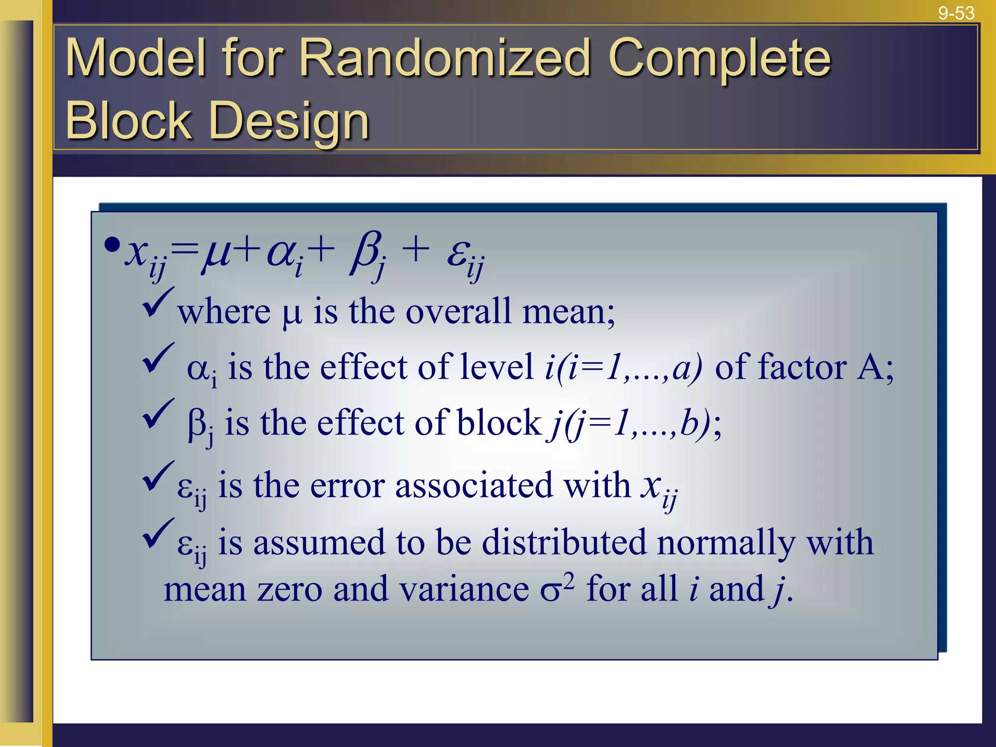
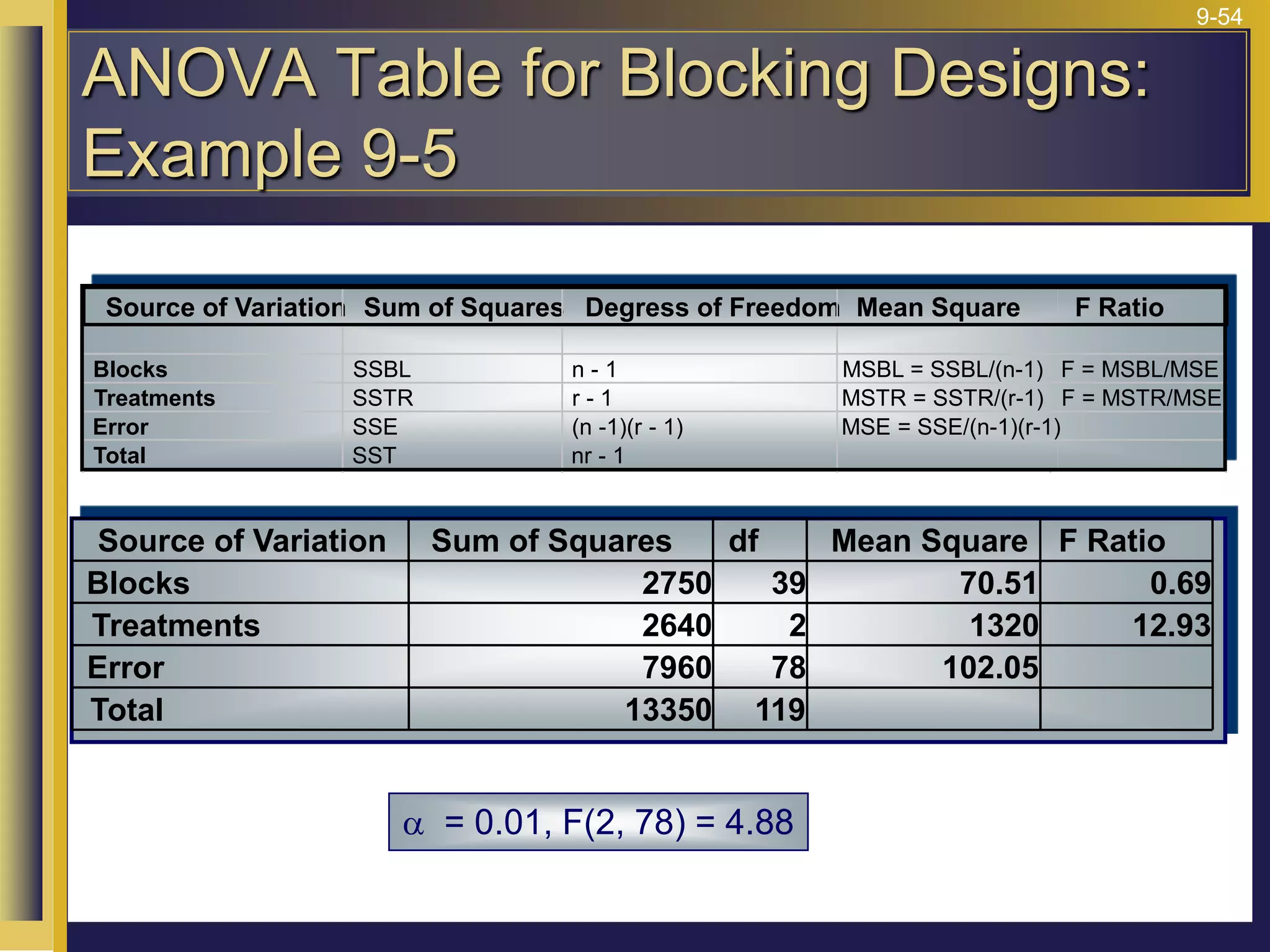
The document provides an overview of analysis of variance (ANOVA) including its purpose, assumptions, computations, and applications. It explains that ANOVA tests whether population means are equal by comparing two estimators of variance - the variation between sample means and the variation within samples. If the null hypothesis that all population means are equal is true, the between-sample variation will be small relative to the within-sample variation. The document outlines the computations and formulas behind ANOVA including definitions of terms like treatment deviations, error deviations, and sums of squares. It also describes how to interpret and report ANOVA results including the F-statistic and ANOVA table.

1. 9-1
STATISTICS

2. 9-2
Chapter 9
Analysis of Variance

3. 9-3
•Using Statistics
•The Hypothesis Test of Analysis of Variance
•The Theory and Computations of ANOVA
•The ANOVA Table and Examples
•Further Analysis
•Models, Factors, and Designs
•Two-Way Analysis of Variance
•Blocking Designs
Analysis of Variance
9

4. 9-4
• Explain the purpose of ANOVA
• Describe the model and computations behind ANOVA
• Explain the test statistic F
• Conduct a 1-way ANOVA
• Report ANOVA results in an ANOVA table
• Apply Tukey test for pair-wise analysis
• Conduct a 2-way ANOVA
• Explain blocking designs
• Apply templates to conduct 1-way and 2-way ANOVA
LEARNING OBJECTIVES
9
After studying this chapter you should be able to:

5. 9-5
• ANOVA (ANalysis Of VAriance) is a statistical
method for determining the existence of
differences among several population means.
ANOVA is designed to detect differences among means
from populations subject to different treatments
ANOVA is a joint test
The equality of several population means is tested
simultaneously or jointly.
ANOVA tests for the equality of several population
means by looking at two estimators of the population
variance (hence, analysis of variance).
9-1 Using Statistics

6. 9-6
• In an analysis of variance:
We have r independent random samples, each one
corresponding to a population subject to a different
treatment.
We have:
 n = n1+ n2+ n3+ ...+nr total observations.
r sample means: x1, x2 , x3 , ... , xr
 These r sample means can be used to calculate an estimator of
the population variance. If the population means are equal,
we expect the variance among the sample means to be small.
r sample variances: s1
2, s2
2, s3
2, ...,sr
2
 These sample variances can be used to find a pooled
estimator of the population variance.
9-2 The Hypothesis Test of
Analysis of Variance

7. 9-7
• We assume independent random sampling from each of the
r populations
• We assume that the r populations under study:
 are normally distributed,
 with means mi that may or may not be equal,
 but with equal variances, si
2.
m1 m2 m3
s
Population 1 Population 2 Population 3
9-2 The Hypothesis Test of Analysis of
Variance (continued): Assumptions

8. 9-8
The test statistic of analysis of variance:
F(r-1, n-r) = Estimate of variance based on means from r samples
Estimate of variance based on all sample observations
That is, the test statistic in an analysis of variance is based on the ratio of
two estimators of a population variance, and is therefore based on the F
distribution, with (r-1) degrees of freedom in the numerator and (n-r)
degrees of freedom in the denominator.
The hypothesis test of analysis of variance:
H0: m1 = m2 = m3 = m4 = ... mr
H1: Not all mi (i = 1, ..., r) are equal
9-2 The Hypothesis Test of Analysis of
Variance (continued)

9. 9-9
x
x
x
When the null hypothesis is true:
We would expect the sample means to be nearly
equal, as in this illustration. And we would
expect the variation among the sample means
(between sample) to be small, relative to the
variation found around the individual sample
means (within sample).
If the null hypothesis is true, the numerator in
the test statistic is expected to be small, relative
to the denominator:
F(r-1, n-r)= Estimate of variance based on means from r samples
Estimate of variance based on all sample observations
H0: m = m = m
When the Null Hypothesis Is True

10. 9-10
x x
x
When the null hypothesis is false:
is equal to but not to ,
is equal to but not to ,
is equal to but not to , or
, , and are all unequal.
m
m
m
m
m
m
m
m
m
m
m
m
In any of these situations, we would not expect the sample means to all be nearly
equal. We would expect the variation among the sample means (between
sample) to be large, relative to the variation around the individual sample means
(within sample).
If the null hypothesis is false, the numerator in the test statistic is expected to be
large, relative to the denominator:
F(r-1, n-r)= Estimate of variance based on means from r samples
Estimate of variance based on all sample observations
When the Null Hypothesis Is False

11. 9-11
•Suppose we have 4 populations, from each of which we
draw an independent random sample, with n1 + n2 + n3
+ n4 = 54. Then our test statistic is:
F(4-1, 54-4)= F(3,50) = Estimate of variance based on means from 4 samples
Estimate of variance based on all 54 sample observations
5
4
3
2
1
0
0.7
0.6
0.5
0.4
0.3
0.2
0.1
0.0
F(3,50)
f
(
F)
FDistributionwith3and 50 Degreesof Freedom
2.79
a=0.05
The nonrejection region (for a=0.05)in this
instance is F  2.79, and the rejection region
is F > 2.79. If the test statistic is less than
2.79 we would not reject the null hypothesis,
and we would conclude the 4 population
means are equal. If the test statistic is
greater than 2.79, we would reject the null
hypothesis and conclude that the four
population means are not equal.
The ANOVA Test Statistic for r = 4 Populations and
n = 54 Total Sample Observations

12. 9-12
Randomly chosen groups of customers were served different types of coffee and asked to rate the
coffee on a scale of 0 to 100: 21 were served pure Brazilian coffee, 20 were served pure Colombian
coffee, and 22 were served pure African-grown coffee.
The resulting test statistic was F = 2.02
others.
the
from
tly
significan
differs
means
population
the
of
any
that
conclude
cannot
we
and
rejected,
be
cannot
0
H
15
.
3
60
,
2
02
.
2
15
.
3
60
,
2
3
63
,
1
3
-
,
1
-
:
is
0.05
=
for
point
critical
The
3
=
r
63
=
22
+
20
+
21
=
n
22
=
3
n
20
=
2
n
21
=
1
n
equal
means
three
all
Not
:
1
H
3
2
1
:
0
H
=

=
=
=


=
=
=
































F
F
F
F
r
n
r
F
a
m
m
m
5
4
3
2
1
0
0.7
0.6
0.5
0.4
0.3
0.2
0.1
0.0
F
f(F)
F Distribution with 2 and 60 Degrees of Freedom
a=0.05
Test Statistic=2.02 F(2,60)=3.15
Example 9-1

13. 9-13
The grand mean, x, is the mean of all n = n1+ n2+ n3+...+ nr observations
in all r samples.
.
j
n
to
1
from
runs
j
thus,
i;
population
from
sample
in the
point with
data
the
denotes
j
subscript
The
r.
to
1
from
runs
and
nt,
or treatme
,
population
the
denotes
i
subscript
The
i.
population
from
sample
e
within th
j
position
in
point
data
particular
the
is
ij
x
where
1
=
1 ij
x
1
=
:
points
data
all
of
mean
the
mean,
grand
The
1 ij
x
=
:
r)
1,2,3,...,
=
(i
i
sample
of
mean
The
i
n
i
n
i
n
j
r
i
i
x
i
n
i
n
j
i
x
r
i
x
n

=

=

=

=
9-3 The Theory and the Computations
of ANOVA: The Grand Mean

14. 9-14
Using the Grand Mean: Table 9-1
If the r population means are different (that is, at
least two of the population means are not equal),
then it is likely that the variation of the data
points about their respective sample means
(within sample variation) will be small relative
to the variation of the r sample means about the
grand mean (between sample variation).
Distance from data point to its sample mean
Distance from sample mean to grand mean
10
5
0
x3=2
x2=11.5
x1=6
x=6.909
Treatment (j) Sample point(j) Value(xij)
I = 1 Triangle 1 4
Triangle 2 5
Triangle 3 7
Triangle 4 8
Mean of Triangles 6
I = 2 Square 1 10
Square 2 11
Square 3 12
Square 4 13
Mean of Squares 11.5
I = 3 Circle 1 1
Circle 2 2
Circle 3 3
Mean of Circ
les 2
Grand mean of all data points 6.909

15. 9-15
We define an as the difference between a data point
and its sample mean. Errors are denoted by , and we have:
We define a as the deviation of a sample mean
from the grand mean. Treatment deviations, t are given by:
i
error deviation
treatment deviation
e
,
The ANOVA principle says:
When the population means are not equal, the “average” error
(within sample) is relatively small compared with the “average”
treatment (between sample) deviation.
The Theory and Computations of ANOVA:
Error Deviation and Treatment Deviation
i
ij
ij
x
x
e 
=
x
x
t i
i

=

16. 9-16
Consider data point x24=13 from table 9-1. The
mean of sample 2 is 11.5, and the grand mean is
6.909, so:
e x x
t x x
Tot t e
Tot x x
24 24 2 13 11 5 1 5
2 2 11 5 6 909 4 591
24 2 24 1 5 4 591 6 091
24 24 13 6 909 6 091
=  =  =
=  =  =
=  =  =
=  =  =
. .
. . .
. . .
. .
or
10
5
0
x2=11.5
x = 6.909
x24=13
Total deviation:
Tot24=x24-x=6.091
Treatment deviation:
t2=x2-x=4.591
Error deviation:
e24=x24-x2=1.5
The total deviation (Totij) is the difference between a data point (xij) and the grand mean (x):
Totij=xij - x
For any data point xij:
Tot = t + e
That is:
Total Deviation = Treatment Deviation + Error Deviation
The Theory and Computations of
ANOVA: The Total Deviation

17. 9-17
Total Deviation = Treatment Deviation + Error Deviation
Squared Deviations
The total deviation is the sum of the treatment deviation and the error deviation:
+ = ( ) ( )
Notice that the sample mean term ( ) cancels out in the above addition, which
simplifies the equation.
2
+
2
= ( )
2
( )
2
t
i
e
ij
x
i
x xij x
i
xij x Totij
x
i
t
i
e
ij
x
i
x xij x
i
Totij xij x
   =  =
  
= 
( )
( )
2 2
The Theory and Computations of
ANOVA: Squared Deviations

18. 9-18
Sums of Squared Deviations
2
+
2
= n
i
( )
2
( )
2
SST = SSTR + SSE
Tot
ij
j
n
j
i
r
n
i
t
i
i
r
e
ij
j
n
j
i
r
x
ij
x
j
n
j
i
r
x
i
x
i
r
x
ij
x
i
j
n
j
i
r
2
1
1 1 1
1
2
1
1 1 1
1
=
=

=

=

=

=


=

=
 
=
  
=

=

( )
The Sum of Squares Principle
The total sum of squares (SST) is the sum of two terms: the sum of
squares for treatment (SSTR) and the sum of squares for error (SSE).
SST = SSTR + SSE
The Theory and Computations of ANOVA:
The Sum of Squares Principle

19. 9-19
SST
SSTR SSE
SST measures the total variation in the data set, the variation of all individual data
points from the grand mean.
SSTR measures the explained variation, the variation of individual sample means
from the grand mean. It is that part of the variation that is possibly expected, or
explained, because the data points are drawn from different populations. It’s the
variation between groups of data points.
SSE measures unexplained variation, the variation within each group that cannot be
explained by possible differences between the groups.
The Theory and Computations of ANOVA:
Picturing The Sum of Squares Principle

20. 9-20
The number of degrees of freedom associated with SST is (n - 1).
n total observations in all r groups, less one degree of freedom
lost with the calculation of the grand mean
The number of degrees of freedom associated with SSTR is (r - 1).
r sample means, less one degree of freedom lost with the
calculation of the grand mean
The number of degrees of freedom associated with SSE is (n-r).
n total observations in all groups, less one degree of freedom
lost with the calculation of the sample mean from each of r groups
The degrees of freedom are additive in the same way as are the sums of squares:
df(total) = df(treatment) + df(error)
(n - 1) = (r - 1) + (n - r)
The Theory and Computations of
ANOVA: Degrees of Freedom

21. 9-21
Recall that the calculation of the sample variance involves the division of the sum of
squared deviations from the sample mean by the number of degrees of freedom. This
principle is applied as well to find the mean squared deviations within the analysis of
variance.
Mean square treatment (MSTR):
Mean square error (MSE):
Mean square total (MST):
(Note that the additive properties of sums of squares do not extend to the mean
squares. MST  MSTR + MSE.
MSTR
SSTR
r
=

( )
1
MSE
SSE
n r
=

( )
MST
SST
n
=

( )
1
The Theory and Computations of
ANOVA: The Mean Squares

22. 9-22
E MSE
E MSTR
ni i
r
i
( )
and
( )
( ) when the null hypothesis is true
> when the null hypothesis is false
where is the mean of population i and is the combined mean of all r populations.
=
= 



=
s
s
m m s
s
m m
2
2
2
1
2
2
That is, the expected mean square error (MSE) is simply the common population variance
(remember the assumption of equal population variances), but the expected treatment sum of
squares (MSTR) is the common population variance plus a term related to the variation of the
individual population means around the grand population mean.
If the null hypothesis is true so that the population means are all equal, the second term in
the E(MSTR) formulation is zero, and E(MSTR) is equal to the common population variance.
The Theory and Computations of
ANOVA: The Expected Mean Squares

23. 9-23
When the null hypothesis of ANOVA is true and all r population means are
equal, MSTR and MSE are two independent, unbiased estimators of the
common population variance s2.
On the other hand, when the null hypothesis is false, then MSTR will tend to
be larger than MSE.
So the ratio of MSTR and MSE can be used as an indicator of the
equality or inequality of the r population means.
This ratio (MSTR/MSE) will tend to be near to 1 if the null hypothesis is
true, and greater than 1 if the null hypothesis is false. The ANOVA test,
finally, is a test of whether (MSTR/MSE) is equal to, or greater than, 1.
Expected Mean Squares and the
ANOVA Principle

24. 9-24
Under the assumptions of ANOVA, the ratio (MSTR/MSE)
possess an F distribution with (r-1) degrees of freedom for the
numerator and (n-r) degrees of freedom for the denominator
when the null hypothesis is true.
The test statistic in analysis of variance:
( - , - )
F
MSTR
MSE
r n r
1
=
The Theory and Computations of
ANOVA: The F Statistic

25. 9-25
( )
2
n
i
( )
2
Critical point ( = 0.01): 8.65
H
0
may be rejected at the 0.01 level
of significance.
SSE x
ij
x
i
j
n
j
i
r
SSTR x
i
x
i
r
MSTR
SSTR
r
MSE
SSTR
n r
F
MSTR
MSE
= 
=
 =
=

= 
=
 =
=

=

=
=

= =
= = =
1
17
1
1
159 9
1
159 9
3 1
79 95
17
8
2 125
2 8
79 95
2 125
37 62
.
.
( )
.
.
( , )
.
.
. .
a
Treatment (i) i j Value (x ij ) (xij -xi ) (xij -xi )2
Triangle 1 1 4 -2 4
Triangle 1 2 5 -1 1
Triangle 1 3 7 1 1
Triangle 1 4 8 2 4
Square 2 1 10 -1.5 2.25
Square 2 2 11 -0.5 0.25
Square 2 3 12 0.5 0.25
Square 2 4 13 1.5 2.25
Circle 3 1 1 -1 1
Circle 3 2 2 0 0
Circle 3 3 3 1 1
73 0 17
Treatment (xi -x) (xi -x)2
ni (xi -x)2
Triangle -0.909 0.826281 3.305124
Square 4.591 21.077281 84.309124
Circle -4.909 124.098281 72.294843
159.909091
9-4 The ANOVA Table and Examples

26. 9-26
Source of
Variation
Sum of
Squares
Degrees of
Freedom Mean Square F Ratio
Treatment SSTR=159.9 (r-1)=2 MSTR=79.95 37.62
Error SSE=17.0 (n-r)=8 MSE=2.125
Total SST=176.9 (n-1)=10 MST=17.69
10
0
0.7
0.6
0.5
0.4
0.3
0.2
0.1
0.0
F(2,8)
f(F)
F Distribution for 2 and 8 Degrees of Freedom
8.65
0.01
Computed test statistic=37.62
The ANOVA Table summarizes the
ANOVA calculations.
In this instance, since the test statistic is
greater than the critical point for an a =
0.01 level of significance, the null
hypothesis may be rejected, and we may
conclude that the means for triangles,
squares, and circles are not all equal.
ANOVA Table

27. 9-27
Template Output

28. 9-28
Club Med has conducted a test to determine whether its Caribbean resorts are equally well liked by
vacationing club members. The analysis was based on a survey questionnaire (general satisfaction,
on a scale from 0 to 100) filled out by a random sample of 40 respondents from each of 5 resorts.
Source of
Variation
Sum of
Squares
Degrees of
Freedom Mean Square F Ratio
Treatment SSTR= 14208 (r-1)= 4 MSTR= 3552 7.04
Error SSE=98356 (n-r)= 195 MSE= 504.39
Total SST=112564 (n-1)= 199 MST= 565.65
Resort Mean Response (x )
i
Guadeloupe 89
Martinique 75
Eleuthra 73
Paradise Island 91
St. Lucia 85
SST=112564 SSE=98356
F(4,200)
F Distribution with 4 and 200 Degrees of Freedom
0
0.7
0.6
0.5
0.4
0.3
0.2
0.1
0.0
f(F)
3.41
0.01
Computed test statistic=7.04
The resultant F
ratio is larger than
the critical point for
a = 0.01, so the
null hypothesis may
be rejected.
Example 9-2: Club Med

29. 9-29
Source of
Variation
Sum of
Squares
Degrees of
Freedom Mean Square F Ratio
Treatment SSTR= 879.3 (r-1)=3 MSTR= 293.1 8.52
Error SSE= 18541.6 (n-r)= 539 MSE=34.4
Total SST= 19420.9 (n-1)=542 MST= 35.83
Given the total number of observations (n = 543), the number of groups
(r = 4), the MSE (34. 4), and the F ratio (8.52), the remainder of the ANOVA
table can be completed. The critical point of the F distribution for a = 0.01
and (3, 400) degrees of freedom is 3.83. The test statistic in this example is
much larger than this critical point, so the p value associated with this test
statistic is less than 0.01, and the null hypothesis may be rejected.
Example 9-3: Job Involvement

30. 9-30
Data ANOVA
Do Not Reject H0 Stop
Reject H0
The sample means are unbiased estimators of the population means.
The mean square error (MSE) is an unbiased estimator of the common
population variance.
Further
Analysis
Confidence Intervals
for Population Means
Tukey Pairwise
Comparisons Test
The ANOVA Diagram
9-5 Further Analysis

31. 9-31
A (1 - ) 100% confidence interval for , the mean of population i:
i
a m
a
a
where t is the value of the distribution with ) degrees of
freedom that cuts off a right - tailed area of
2
.
2
a
x t
MSE
n
i
i

2
t (n- r
x t
MSE
n
x x
i
i
i i
 =  = 
 =
 =
 =
 =
 =
a
2
1 96
504 39
40
6 96
89 6 96 82 04 95 96]
75 6 96 68 04 81 96]
73 6 96 66 04 79 96]
91 6 96 84 04 97 96]
85 6 96 78 04 91 96]
.
.
.
. [ . , .
. [ . , .
. [ . , .
. [ . , .
. [ . , .
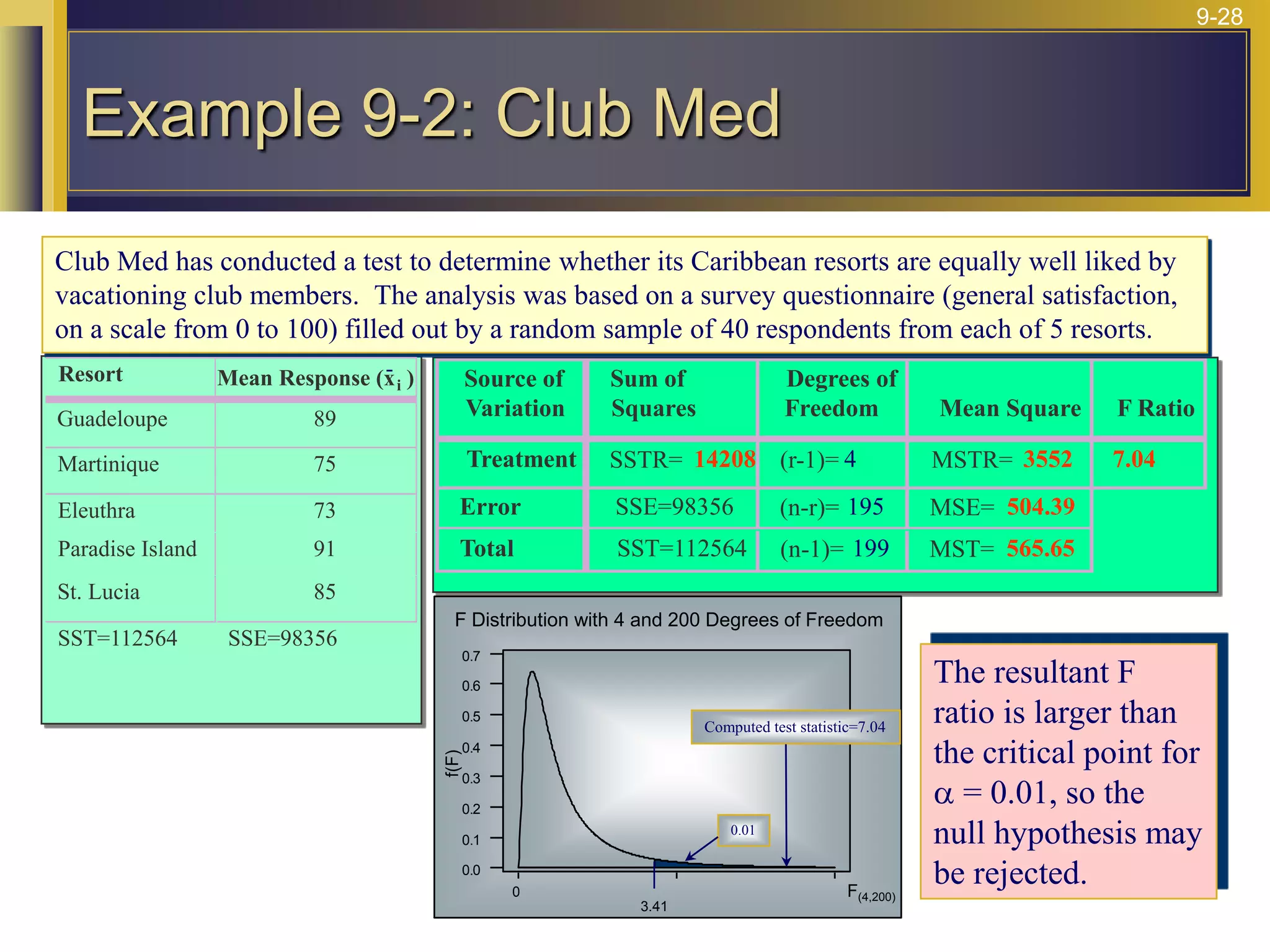
Resort Mean Response (x i)
Guadeloupe 89
Martinique 75
Eleuthra 73
Paradise Island 91
St. Lucia 85
SST = 112564 SSE = 98356
ni = 40 n = (5)(40) = 200
MSE = 504.39
Confidence Intervals for Population
Means

32. 9-32
The Tukey Pairwise Comparison test, or Honestly Significant Differences (MSD) test, allows us
to compare every pair of population means with a single level of significance.
It is based on the studentized range distribution, q, with r and (n-r) degrees of freedom.
The critical point in a Tukey Pairwise Comparisons test is the Tukey Criterion:
where ni is the smallest of the r sample sizes.
The test statistic is the absolute value of the difference between the appropriate sample means, and
the null hypothesis is rejected if the test statistic is greater than the critical point of the Tukey
Criterion
T q
MSE
ni
= a
 
N ote that there are
r
2
pairs of population m eans to com pare. For exam ple, if = :
H 0 H 0 H 0
H 1 H 1 H 1
=

= = =
  
r
r
r
!
!( ) !
: : :
: : :
2 2
3
1 2 1 3 2 3
1 2 1 3 2 3
m m m m m m
m m m m m m
The Tukey Pairwise-Comparisons
Test

33. 9-33
The test statistic for each pairwise test is the absolute difference between the appropriate
sample means.
i Resort Mean I. H0: m1 = m2 VI. H0: m2 = m4
1 Guadeloupe 89 H1: m1  m2 H1: m2  m4
2 Martinique 75 |89-75|=14>13.7* |75-91|=16>13.7*
3 Eleuthra 73 II. H0: m1 = m3 VII. H0: m2 = m5
4 Paradise Is. 91 H1: m1  m3 H1: m2  m5
5 St. Lucia 85 |89-73|=16>13.7* |75-85|=10<13.7
III. H0: m1 = m4 VIII. H0: m3 = m4
The critical point T0.05 for H1: m1  m4 H1: m3  m4
r=5 and (n-r)=195 |89-91|=2<13.7 |73-91|=18>13.7*
degrees of freedom is: IV. H0: m1 = m5 IX. H0: m3 = m5
H1: m1  m5 H1: m3  m5
|89-85|=4<13.7 |73-85|=12<13.7
V. H0: m2 = m3 X. H0: m4 = m5
H1: m2  m3 H1: m4  m5
|75-73|=2<13.7 |91-85|= 6<13.7
Reject the null hypothesis if the absolute value of the difference between the sample means
is greater than the critical value of T. (The hypotheses marked with * are rejected.)
T q
MSE
ni
=
= =
a
386
504 4
40
13 7
.
.
.
The Tukey Pairwise Comparison Test:
The Club Med Example

34. 9-34
We rejected the null hypothesis which compared the means of populations 1
and 2, 1 and 3, 2 and 4, and 3 and 4. On the other hand, we accepted the null
hypotheses of the equality of the means of populations 1 and 4, 1 and 5, 2
and 3, 2 and 5, 3 and 5, and 4 and 5.
The bars indicate the three groupings of populations with possibly equal
means: 2 and 3; 2, 3, and 5; and 1, 4, and 5.
m
1
m
2
m
3
m
4
m
5
Picturing the Results of a Tukey Pairwise
Comparisons Test: The Club Med Example

35. 9-35
Picturing the Results of a Tukey Pairwise
Comparisons Test: The Club Med Example

36. 9-36
• A statistical model is a set of equations and assumptions
that capture the essential characteristics of a real-world
situation
The one-factor ANOVA model:
xij=mi+eij=m+ai+eij
where eij is the error associated with the jth member of
the ith population. The errors are assumed to be
normally distributed with mean 0 and variance s2.
9-6 Models, Factors and Designs

37. 9-37
• A factor is a set of populations or treatments of a single kind. For
example:
One factor models based on sets of resorts, types of airplanes, or
kinds of sweaters
Two factor models based on firm and location
Three factor models based on color and shape and size of an ad.
• Fixed-Effects and Random Effects
A fixed-effects model is one in which the levels of the factor under
study (the treatments) are fixed in advance. Inference is valid only
for the levels under study.
A random-effects model is one in which the levels of the factor
under study are randomly chosen from an entire population of levels
(treatments). Inference is valid for the entire population of levels.
9-6 Models, Factors and Designs
(Continued)

38. 9-38
• A completely-randomized design is one in which the
elements are assigned to treatments completely at random.
That is, any element chosen for the study has an equal
chance of being assigned to any treatment.
• In a blocking design, elements are assigned to treatments
after first being collected into homogeneous groups.
In a completely randomized block design, all members of each
block (homogeneous group) are randomly assigned to the treatment
levels.
In a repeated measures design, each member of each block is
assigned to all treatment levels.
Experimental Design

39. 9-39
• In a two-way ANOVA, the effects of two factors or treatments can be investigated
simultaneously. Two-way ANOVA also permits the investigation of the effects of
either factor alone and of the two factors together.
The effect on the population mean that can be attributed to the levels of either factor alone
is called a main effect.
An interaction effect between two factors occurs if the total effect at some pair of levels of
the two factors or treatments differs significantly from the simple addition of the two main
effects. Factors that do not interact are called additive.
• Three questions answerable by two-way ANOVA:
Are there any factor A main effects?
Are there any factor B main effects?
Are there any interaction effects between factors A and B?
• For example, we might investigate the effects on vacationers’ ratings of resorts by
looking at five different resorts (factor A) and four different resort attributes (factor
B). In addition to the five main factor A treatment levels and the four main factor B
treatment levels, there are (5*4=20) interaction treatment levels.3
9-7 Two-Way Analysis of Variance

40. 9-40
•xijk=m+ai+ bj + (abij + eijk
where m is the overall mean;
 ai is the effect of level i(i=1,...,a) of factor A;
 bj is the effect of level j(j=1,...,b) of factor B;
 abjj is the interaction effect of levels i and j;
 ejjk is the error associated with the kth data point from
level i of factor A and level j of factor B.
 ejjk is assumed to be distributed normally with mean
zero and variance s2 for all i, j, and k.
The Two-Way ANOVA Model

41. 9-41
Guadeloupe Martinique Eleuthra
Paradise
Island St. Lucia
Friendship n11 n21 n31 n41 n51
Sports n12 n22 n32 n42 n52
Culture n13 n23 n33 n43 n53
Excitement n14 n24 n34 n44 n54
Factor A: Resort
Factor
B:
Attribute
Resort
R
a
ting
Graphical Display of Effects
Eleuthra
Martinique
St. Lucia
Guadeloupe
Paradise island
Friendship
Excitement
Sports
Culture
Eleuthra/sports interaction:
Combined effect greater than
additive main effects
Sports
Friendship
Attribute
Resort
Excitement
Culture
Rating
Eleuthra
Martinique
St. Lucia
Guadeloupe
Paradise Island
Two-Way ANOVA Data Layout:
Club Med Example

42. 9-42
•Factor A main effects test:
H0: ai= 0 for all i=1,2,...,a
H1: Not all ai are 0
•Factor B main effects test:
H0: bj= 0 for all j=1,2,...,b
H1: Not all bi are 0
•Test for (AB) interactions:
H0: abij= 0 for all i=1,2,...,a and j=1,2,...,b
H1: Not all abij are 0
Hypothesis Tests a Two-Way ANOVA

43. 9-43
 In a two-way ANOVA:
xijk=m+ai+ bj + (abijk + eijk
 SST = SSTR +SSE
 SST = SSA + SSB +SS(AB)+SSE
SST SSTR SSE
x x x x x x
SSTR SSA SSB SS AB
x
i
x x
j
x x
ij
x
i
x
j
x
= 



 = 


  



=  
=   





    



( ) ( ) ( )
( )
( ) ( ) ( )
2 2 2
2 2 2
Sums of Squares

44. 9-44
Source of
Variation
Sum of
Squares
Degrees
of Freedom Mean Square F Ratio
Factor A SSA a-1
MSA
SSA
a
=
1
F
MSA
MSE
=
Factor B SSB b-1
MSB
SSB
b
=
1
F
MSB
MSE
=
Interaction SS(AB) (a-1)(b-1)
MS AB
SS AB
a b
( )
( )
( )( )
=
 
1 1
F
MS AB
MSE
=
( )
Error SSE ab(n-1)
MSE
SSE
ab n
=

( )
1
Total SST abn-1
A Main Effect Test: F(a-1,ab(n-1)) B Main Effect Test: F(b-1,ab(n-1))
(AB) Interaction Effect Test: F((a-1)(b-1),ab(n-1))
The Two-Way ANOVA Table

45. 9-45
Source of
Variation
Sum of
Squares
Degrees
of Freedom Mean Square F Ratio
Location 1824 2 912 8.94
Artist 2230 2 1115 10.93
Interaction 804 4 201 1.97
Error 8262 81 102
Total 13120 89
a =0.01, F(2,81)=4.88  Both main effect null hypotheses are rejected.
a=0.05, F(2,81)=2.48  Interaction effect null hypotheses are not rejected.
Example 9-4: Two-Way ANOVA
(Location and Artist)

46. 9-46
6
5
4
3
2
1
0
0.7
0.6
0.5
0.4
0.3
0.2
0.1
0.0
F
f(F)
FDistributionwith2 and 81 Degrees of Freedom
F0.01=4.88
a=0.01
Location test statistic=8.94
Artist test statistic=10.93
6
5
4
3
2
1
0
0.7
0.6
0.5
0.4
0.3
0.2
0.1
0.0 F
f(F)
F Distribution with 4 and 81 Degrees of Freedom
Interaction test statistic=1.97
a=0.05
F0.05=2.48
Hypothesis Tests

47. 9-47
Kimball’s Inequality gives an upper limit on the true probability of at least
one Type I error in the three tests of a two-way analysis:
a  1- (1-a1) (1-a2) (1-a3)
Tukey Criterion for factor A:
where the degrees of freedom of the q distribution are now a and ab(n-1). Note
that MSE is divided by bn.
T q
MSE
bn
= a
Overall Significance Level and Tukey
Method for Two-Way ANOVA

48. 9-48
Template for a Two-Way ANOVA

49. 9-49
Source of
Variation
Sum of
Squares
Degrees
of Freedom Mean Square F Ratio
Factor A SSA a-1 MSA
SSA
a
=
1 F
MSA
MSE
=
Factor B SSB b-1
MSB
SSB
b
=
1
F
MSB
MSE
=
Factor C SSC c-1
MSC
SSC
c
=
1
F
MSC
MSE
=
Interaction
(AB)
SS(AB) (a-1)(b-1)
MS AB
SS AB
a b
( )
( )
( )( )
=
 
1 1
F
MS AB
MSE
=
( )
Interaction
(AC)
SS(AC) (a-1)(c-1)
MS AC
SS AC
a c
( )
( )
( )( )
=
 
1 1
F
MS AC
MSE
=
( )
Interaction
(BC)
SS(BC) (b-1)(c-1)
MS BC
SS BC
b c
( )
( )
( )( )
=
 
1 1
F
MS BC
MSE
= ( )
Interaction
(ABC)
SS(ABC) (a-1)(b-1)(c-1) MS ABC
SS ABC
a b c
( )
( )
( )( )( )
=
  
1 1 1
F
MS ABC
MSE
=
( )
Error SSE abc(n-1) MSE
SSE
abc n
=

( )
1
Total SST abcn-1
Extension of ANOVA to Three Factors

50. 9-50
• The case of one data point in every cell presents a
problem in two-way ANOVA.
• There will be no degrees of freedom for the error term.
• What can be done?
• If we can assume that there are no interactions between
the main effects, then we can use SS(AB) and its
associated degrees of freedom (a – 1)(b – 1) in place of
SSE and its degrees of freedom.
• We can then conduct main effects tests using MS(AB).
• See the next slide for the ANOVA table.
Two-Way ANOVA with One
Observation per Cell

51. 9-51
Two-Way ANOVA with One
Observation per Cell
Source of
Variation
Sum of
Squares
Degrees of
Freedom
Mean Square F Ratio
Factor A SSA a - 1
Factor B SSB b - 1
“Error” SS(AB) (a – 1)(b –
1)
Total SST ab - 1
1

=
a
SSA
MSA
1

=
b
SSB
MSB
)
1
)(
1
(
)
(
)
(


=
b
a
AB
SS
AB
MS
)
(AB
MS
MSA
F =
)
(AB
MS
MSB
F =

52. 9-52
• A block is a homogeneous set of subjects, grouped to
minimize within-group differences.
• A competely-randomized design is one in which the
elements are assigned to treatments completely at
random. That is, any element chosen for the study has an
equal chance of being assigned to any treatment.
• In a blocking design, elements are assigned to treatments
after first being collected into homogeneous groups.
In a completely randomized block design, all members of each
block (homogenous group) are randomly assigned to the
treatment levels.
In a repeated measures design, each member of each block is
assigned to all treatment levels.
9-8 Blocking Designs

53. 9-53
•xij=m+ai+ bj + eij
where m is the overall mean;
 ai is the effect of level i(i=1,...,a) of factor A;
 bj is the effect of block j(j=1,...,b);
eij is the error associated with xij
eij is assumed to be distributed normally with
mean zero and variance s2 for all i and j.
Model for Randomized Complete
Block Design

54. 9-54
ANOVA Table for Blocking Designs:
Example 9-5
Source of Variation Sum of Squares df Mean Square F Ratio
Blocks 2750 39 70.51 0.69
Treatments 2640 2 1320 12.93
Error 7960 78 102.05
Total 13350 119
a = 0.01, F(2, 78) = 4.88
Source of Variation Sum of Squares Degress of Freedom Mean Square F Ratio
Blocks SSBL n - 1 MSBL = SSBL/(n-1) F = MSBL/MSE
Treatments SSTR r - 1 MSTR = SSTR/(r-1) F = MSTR/MSE
Error SSE (n -1)(r - 1)
Total SST nr - 1
MSE = SSE/(n-1)(r-1)

55. 9-55
Template for the Randomized
Complete Block Design