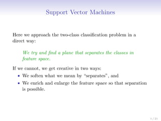
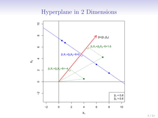
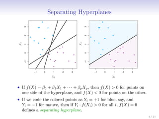
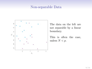
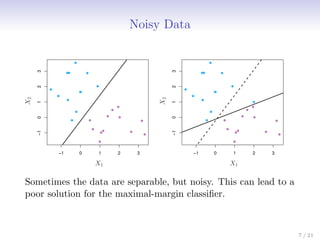
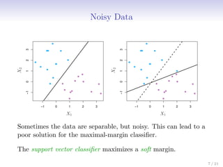
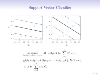
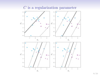
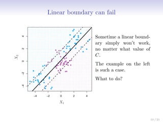
This document discusses support vector machines (SVMs), focusing on the two-class classification problem, hyperplanes, and the concept of maximal margin classifiers. It describes techniques for handling non-separable data, noisy data, and the use of feature expansions and kernels to achieve non-linear decision boundaries. Additionally, it covers how to extend SVMs to classify more than two classes using strategies like one-versus-all and one-versus-one methods.

1. Support Vector Machines
Here we approach the two-class classification problem in a
direct way:
We try and find a plane that separates the classes in
feature space.
If we cannot, we get creative in two ways:
• We soften what we mean by “separates”, and
• We enrich and enlarge the feature space so that separation
is possible.
1 / 21

2. What is a Hyperplane?
• A hyperplane in p dimensions is a flat affine subspace of
dimension p − 1.
• In general the equation for a hyperplane has the form
β0 + β1X1 + β2X2 + . . . + βpXp = 0
• In p = 2 dimensions a hyperplane is a line.
• If β0 = 0, the hyperplane goes through the origin,
otherwise not.
• The vector β = (β1, β2, · · · , βp) is called the normal vector
— it points in a direction orthogonal to the surface of a
hyperplane.
2 / 21

3. Hyperplane in 2 Dimensions
−2 0 2 4 6 8 10
−2
0
2
4
6
8
10
X1
X
2
●
●
●
●
●
β=(β1,β2)
β1X1+β2X2−6=0
β1X1+β2X2−6=1.6
●
β1X1+β2X2−6=−4
β1 = 0.8
β2 = 0.6
3 / 21

4. Separating Hyperplanes
−1 0 1 2 3
−1
0
1
2
3
−1 0 1 2 3
−1
0
1
2
3
X1
X1
X
2
X
2
• If f(X) = β0 + β1X1 + · · · + βpXp, then f(X) > 0 for points on
one side of the hyperplane, and f(X) < 0 for points on the other.
• If we code the colored points as Yi = +1 for blue, say, and
Yi = −1 for mauve, then if Yi · f(Xi) > 0 for all i, f(X) = 0
defines a separating hyperplane.
4 / 21

5. Maximal Margin Classifier
Among all separating hyperplanes, find the one that makes the
biggest gap or margin between the two classes.
−1 0 1 2 3
−1
0
1
2
3
X1
X
2
Constrained optimization problem
maximize
β0,β1,...,βp
M
subject to
p
X
j=1
β2
j = 1,
yi(β0 + β1xi1 + . . . + βpxip) ≥ M
for all i = 1, . . . , N.
5 / 21

6. Maximal Margin Classifier
Among all separating hyperplanes, find the one that makes the
biggest gap or margin between the two classes.
−1 0 1 2 3
−1
0
1
2
3
X1
X
2
Constrained optimization problem
maximize
β0,β1,...,βp
M
subject to
p
X
j=1
β2
j = 1,
yi(β0 + β1xi1 + . . . + βpxip) ≥ M
for all i = 1, . . . , N.
This can be rephrased as a convex quadratic program, and
solved efficiently. The function svm() in package e1071 solves
this problem efficiently 5 / 21

7. Non-separable Data
0 1 2 3
−1.0
−0.5
0.0
0.5
1.0
1.5
2.0
X1
X
2
The data on the left are
not separable by a linear
boundary.
This is often the case,
unless N < p.
6 / 21

8. Noisy Data
−1 0 1 2 3
−1
0
1
2
3
−1 0 1 2 3
−1
0
1
2
3
X1
X1 X
2
X
2
Sometimes the data are separable, but noisy. This can lead to a
poor solution for the maximal-margin classifier.
7 / 21

9. Noisy Data
−1 0 1 2 3
−1
0
1
2
3
−1 0 1 2 3
−1
0
1
2
3
X1
X1 X
2
X
2
Sometimes the data are separable, but noisy. This can lead to a
poor solution for the maximal-margin classifier.
The support vector classifier maximizes a soft margin.
7 / 21

10. Support Vector Classifier
−0.5 0.0 0.5 1.0 1.5 2.0 2.5
−1
0
1
2
3
4
1
2
3
4 5
6
7
8
9
10
−0.5 0.0 0.5 1.0 1.5 2.0 2.5
−1
0
1
2
3
4
1
2
3
4 5
6
7
8
9
10
11
12
X1
X1
X
2
X
2
maximize
β0,β1,...,βp,1,...,n
M subject to
p
X
j=1
β2
j = 1,
yi(β0 + β1xi1 + β2xi2 + . . . + βpxip) ≥ M(1 − i),
i ≥ 0,
n
X
i=1
i ≤ C,
8 / 21

11. C is a regularization parameter
−1 0 1 2
−3
−2
−1
0
1
2
3
−1 0 1 2
−3
−2
−1
0
1
2
3
−1 0 1 2
−3
−2
−1
0
1
2
3
−1 0 1 2
−3
−2
−1
0
1
2
3
X1
X1
X1
X1
X
2
X
2
X
2
X
2
9 / 21

12. Linear boundary can fail
4 −4 −2 0 2 4
−4
−2
0
2
4
X1
X
2
Sometime a linear bound-
ary simply won’t work,
no matter what value of
C.
The example on the left
is such a case.
What to do?
10 / 21

13. Feature Expansion
• Enlarge the space of features by including transformations;
e.g. X2
1 , X3
1 , X1X2, X1X2
2 ,. . .. Hence go from a
p-dimensional space to a M p dimensional space.
• Fit a support-vector classifier in the enlarged space.
• This results in non-linear decision boundaries in the
original space.
11 / 21

14. Feature Expansion
• Enlarge the space of features by including transformations;
e.g. X2
1 , X3
1 , X1X2, X1X2
2 ,. . .. Hence go from a
p-dimensional space to a M p dimensional space.
• Fit a support-vector classifier in the enlarged space.
• This results in non-linear decision boundaries in the
original space.
Example: Suppose we use (X1, X2, X2
1 , X2
2 , X1X2) instead of
just (X1, X2). Then the decision boundary would be of the form
β0 + β1X1 + β2X2 + β3X2
1 + β4X2
2 + β5X1X2 = 0
This leads to nonlinear decision boundaries in the original space
(quadratic conic sections).
11 / 21

15. Cubic Polynomials
Here we use a basis
expansion of cubic poly-
nomials
From 2 variables to 9
The support-vector clas-
sifier in the enlarged
space solves the problem
in the lower-dimensional
space
−4 −2 0 2 4
−4
−2
0
2
4
−4
−2
0
2
4
X1
X
2
X
2
12 / 21

16. Cubic Polynomials
Here we use a basis
expansion of cubic poly-
nomials
From 2 variables to 9
The support-vector clas-
sifier in the enlarged
space solves the problem
in the lower-dimensional
space
−4 −2 0 2 4
−4
−2
0
2
4
−4
−2
0
2
4
X1
X
2
X
2
β0+β1X1+β2X2+β3X2
1 +β4X2
2 +β5X1X2+β6X3
1 +β7X3
2 +β8X1X2
2 +β9X2
1 X2 = 0
12 / 21

17. Nonlinearities and Kernels
• Polynomials (especially high-dimensional ones) get wild
rather fast.
• There is a more elegant and controlled way to introduce
nonlinearities in support-vector classifiers — through the
use of kernels.
• Before we discuss these, we must understand the role of
inner products in support-vector classifiers.
13 / 21

18. Inner products and support vectors
hxi, xi0 i =
p
X
j=1
xijxi0j — inner product between vectors
14 / 21

19. Inner products and support vectors
hxi, xi0 i =
p
X
j=1
xijxi0j — inner product between vectors
• The linear support vector classifier can be represented as
f(x) = β0 +
n
X
i=1
αihx, xii — n parameters
14 / 21

20. Inner products and support vectors
hxi, xi0 i =
p
X
j=1
xijxi0j — inner product between vectors
• The linear support vector classifier can be represented as
f(x) = β0 +
n
X
i=1
αihx, xii — n parameters
• To estimate the parameters α1, . . . , αn and β0, all we need
are the n
2
inner products hxi, xi0 i between all pairs of
training observations.
14 / 21

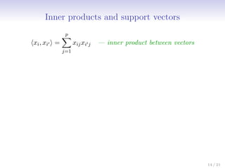
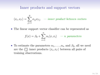
21. Inner products and support vectors
hxi, xi0 i =
p
X
j=1
xijxi0j — inner product between vectors
• The linear support vector classifier can be represented as
f(x) = β0 +
n
X
i=1
αihx, xii — n parameters
• To estimate the parameters α1, . . . , αn and β0, all we need
are the n
2
inner products hxi, xi0 i between all pairs of
training observations.
It turns out that most of the α̂i can be zero:
f(x) = β0 +
X
i∈S
α̂ihx, xii
S is the support set of indices i such that α̂i 0. [see slide 8]
14 / 21

22. Kernels and Support Vector Machines
• If we can compute inner-products between observations, we
can fit a SV classifier. Can be quite abstract!
15 / 21

23. Kernels and Support Vector Machines
• If we can compute inner-products between observations, we
can fit a SV classifier. Can be quite abstract!
• Some special kernel functions can do this for us. E.g.
K(xi, xi0 ) =

1 +
p
X
j=1
xijxi0j


d
computes the inner-products needed for d dimensional
polynomials — p+d
d
basis functions!
15 / 21

24. Kernels and Support Vector Machines
• If we can compute inner-products between observations, we
can fit a SV classifier. Can be quite abstract!
• Some special kernel functions can do this for us. E.g.
K(xi, xi0 ) =

1 +
p
X
j=1
xijxi0j


d
computes the inner-products needed for d dimensional
polynomials — p+d
d
basis functions!
Try it for p = 2 and d = 2.
15 / 21

25. Kernels and Support Vector Machines
• If we can compute inner-products between observations, we
can fit a SV classifier. Can be quite abstract!
• Some special kernel functions can do this for us. E.g.
K(xi, xi0 ) =

1 +
p
X
j=1
xijxi0j


d
computes the inner-products needed for d dimensional
polynomials — p+d
d
basis functions!
Try it for p = 2 and d = 2.
• The solution has the form
f(x) = β0 +
X
i∈S
α̂iK(x, xi).
15 / 21

26. Radial Kernel
K(xi, xi0 ) = exp(−γ
p
X
j=1
(xij − xi0j)2
).
4 −4 −2 0 2 4
−4
−2
0
2
4
X1
X
2
f(x) = β0+
X
i∈S
α̂iK(x, xi)
Implicit feature space;
very high dimensional.
Controls variance by
squashing down most
dimensions severely
16 / 21

27. Example: Heart Data
False positive rate
True
positive
rate
0.0 0.2 0.4 0.6 0.8 1.0
0.0
0.2
0.4
0.6
0.8
1.0
Support Vector Classifier
LDA
False positive rate
True
positive
rate 0.0 0.2 0.4 0.6 0.8 1.0
0.0
0.2
0.4
0.6
0.8
1.0
Support Vector Classifier
SVM: γ=10−3
SVM: γ=10−2
SVM: γ=10−1
ROC curve is obtained by changing the threshold 0 to threshold
t in ˆ
f(X) t, and recording false positive and true positive
rates as t varies. Here we see ROC curves on training data.
17 / 21

28. Example continued: Heart Test Data
False positive rate
True
positive
rate
0.0 0.2 0.4 0.6 0.8 1.0
0.0
0.2
0.4
0.6
0.8
1.0
Support Vector Classifier
LDA
False positive rate
True
positive
rate
0.0 0.2 0.4 0.6 0.8 1.0
0.0
0.2
0.4
0.6
0.8
1.0
Support Vector Classifier
SVM: γ=10−3
SVM: γ=10−2
SVM: γ=10−1
18 / 21

29. SVMs: more than 2 classes?
The SVM as defined works for K = 2 classes. What do we do if
we have K 2 classes?
19 / 21

30. SVMs: more than 2 classes?
The SVM as defined works for K = 2 classes. What do we do if
we have K 2 classes?
OVA One versus All. Fit K different 2-class SVM
classifiers ˆ
fk(x), k = 1, . . . , K; each class versus
the rest. Classify x∗ to the class for which ˆ
fk(x∗)
is largest.
19 / 21

31. SVMs: more than 2 classes?
The SVM as defined works for K = 2 classes. What do we do if
we have K 2 classes?
OVA One versus All. Fit K different 2-class SVM
classifiers ˆ
fk(x), k = 1, . . . , K; each class versus
the rest. Classify x∗ to the class for which ˆ
fk(x∗)
is largest.
OVO One versus One. Fit all K
2
pairwise classifiers
ˆ
fk`(x). Classify x∗ to the class that wins the most
pairwise competitions.
19 / 21

32. SVMs: more than 2 classes?
The SVM as defined works for K = 2 classes. What do we do if
we have K 2 classes?
OVA One versus All. Fit K different 2-class SVM
classifiers ˆ
fk(x), k = 1, . . . , K; each class versus
the rest. Classify x∗ to the class for which ˆ
fk(x∗)
is largest.
OVO One versus One. Fit all K
2
pairwise classifiers
ˆ
fk`(x). Classify x∗ to the class that wins the most
pairwise competitions.
Which to choose? If K is not too large, use OVO.
19 / 21

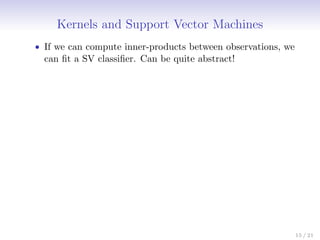
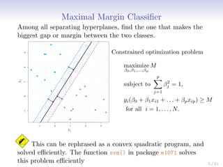
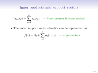
33. Support Vector versus Logistic Regression?
With f(X) = β0 + β1X1 + . . . + βpXp can rephrase
support-vector classifier optimization as
minimize
β0,β1,...,βp



n
X
i=1
max [0, 1 − yif(xi)] + λ
p
X
j=1
β2
j



−6 −4 −2 0 2
0
2
4
6
8
Loss
SVM Loss
Logistic Regression Loss
yi(β0 + β1xi1 + . . . + βpxip)
This has the form
loss plus penalty.
The loss is known as the
hinge loss.
Very similar to “loss” in
logistic regression (negative
log-likelihood).
20 / 21

34. Which to use: SVM or Logistic Regression
• When classes are (nearly) separable, SVM does better than
LR. So does LDA.
• When not, LR (with ridge penalty) and SVM very similar.
• If you wish to estimate probabilities, LR is the choice.
• For nonlinear boundaries, kernel SVMs are popular. Can
use kernels with LR and LDA as well, but computations
are more expensive.
21 / 21