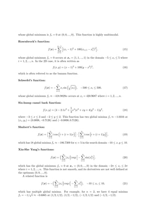
This document provides a list of commonly used test functions for validating new optimization algorithms. It describes 24 test functions, including functions originally developed by De Jong, Griewank, Rastrigin, and Rosenbrock. The test functions have various properties like being unimodal, multimodal, convex, or stochastic. They serve as benchmarks for comparing how well new algorithms can find the optimal value for problems with different characteristics.

1. arXiv:1008.0549v1 [math.OC] 3 Aug 2010
Test Problems in Optimization
Xin-She Yang
Department of Engineering, University of Cambridge,
Cambridge CB2 1PZ, UK
Abstract
Test functions are important to validate new optimization algorithms
and to compare the performance of various algorithms. There are many
test functions in the literature, but there is no standard list or set of test
functions one has to follow. New optimization algorithms should be tested
using at least a subset of functions with diverse properties so as to make
sure whether or not the tested algorithm can solve certain type of opti-mization
efficiently. Here we provide a selected list of test problems for
unconstrained optimization.
Citation detail:
X.-S. Yang, Test problems in optimization, in: Engineering Optimization: An Introduc-tion
with Metaheuristic Applications (Eds Xin-She Yang), John Wiley & Sons, (2010).

2. In order to validate any new optimization algorithm, we have to validate it against
standard test functions so as to compare its performance with well-established or existing
algorithms. There are many test functions, so there is no standard list or set of test functions
one has to follow. However, various test functions do exist, so new algorithms should be
tested using at least a subset of functions with diverse properties so as to make sure whether
or not the tested algorithm can solve certain type of optimization efficiently.
In this appendix, we will provide a subset of commonly used test functions with simple
bounds as constraints, though they are often listed as unconstrained problems in literature.
We will list the function form f(x), its search domain, optimal solutions x and/or optimal
objective value f. Here, we use x = (x1, ..., xn)T where n is the dimension.
Ackley’s function:
f(x) = −20 exp h −
1
5
vuut
1
n
n
Xi
=1
x2i
i − exp h 1
n
n
Xi
=1
cos(2xi)i + 20 + e, (1)
where n = 1, 2, ..., and −32.768 xi 32.768 for i = 1, 2, ..., n. This function has the
global minimum f = 0 at x = (0, 0, ..., 0).
De Jong’s functions: The simplest of De Jong’s functions is the so-called sphere function
f(x) =
n
Xi
=1
x2i
, −5.12 xi 5.12, (2)
whose global minimum is obviously f = 0 at (0, 0, ..., 0). This function is unimodal and
convex. A related function is the so-called weighted sphere function or hyper-ellipsoid
function
f(x) =
n
Xi
=1
ix2i
, −5.12 xi 5.12, (3)
which is also convex and unimodal with a global minimum f = 0 at x = (0, 0, ..., 0).
Another related test function is the sum of different power function
f(x) =
n
=1 |xi|i+1, −1 xi 1, (4)
Xi
which has a global minimum f = 0 at (0, 0, ..., 0).
Easom’s function:
f(x) = −cos(x) cos(y) exp h − (x − )2 + (y − )2i, (5)
whose global minimum is f = −1 at x = (, ) within −100 x, y 100. It has many
local minima. Xin-She Yang extended in 2008 this function to n dimensions, and we have
f(x) = −(−1)n
n
Y
i=1
cos2(xi) exp h −
n
Xi
=1
(xi − )2i, (6)
whose global minimum f = −1 occurs at x = (, , ..., ). Here the domain is −2
xi 2 where i = 1, 2, ..., n.

3. Equality-Constrained Function:
f(x) = −(pn)n
n
Y
i=1
xi, (7)
subject to an equality constraint (a hyper-sphere)
n
Xi
=1
x2i
= 1. (8)
The global minimum f = −1 of f(x) occurs at x(1/pn, ..., 1/pn) within the domain
0 xi 1 for i = 1, 2, ..., n.
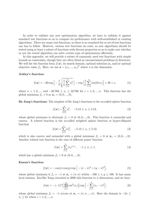
Griewank’s function:
f(x) =
1
4000
n
Xi
=1
x2i
−
n
Y
i=1
cos(
xi pi
) + 1, −600 xi 600, (9)
whose global minimum is f = 0 at x = (0, 0, ..., 0). This function is highly multimodal.
Michaelwicz’s function:
f(x) = −
n
Xi
=1
sin(xi) · h sin(
ix2i
)i2m
, (10)
where m = 10, and 0 xi for i = 1, 2, ..., n. In 2D case, we have
f(x, y) = −sin(x) sin20(
x2
) − sin(y) sin20(
2y2
), (11)
where (x, y) 2 [0, 5] × [0, 5]. This function has a global minimum f −1.8013 at
x = (x, y) = (2.20319, 1.57049).
Perm Functions:
f(x) =
n
X
j=1
n
n
Xi
=1
(ij +

4. )h(
xi
i
)j − 1io, (

5. 0), (12)
which has the global minimum f = 0 at x = (1, 2, ..., n) in the search domain −n xi n
for i = 1, ..., n. A related function
f(x) =
n
X
j=1
n
n
Xi
=1
(i +

6. )hxj
i − (
1
i
)jio2
, (13)
has the global minimum f = 0 at (1, 1/2, 1/3, ..., 1/n) within the bounds −1 xi 1 for
all i = 1, 2, ..., n. As