The document discusses approximations of areas under curves using the trapezoidal rule. It shows the general trapezoidal rule formula for approximating the area under a curve between two points by dividing the area into trapezoids. An example is provided to demonstrate applying the trapezoidal rule with 4 intervals to estimate the area under the curve y = (4 - x)^(1/2) from x = 0 to x = 2, giving an answer of 2.996 units^2 correct to 3 decimal places.
The document describes the trapezoidal rule for approximating the area under a curve. The trapezoidal rule works by dividing the area into trapezoid sections and summing their individual areas. In general, the area is approximated as the average of the initial and final y-values plus twice the sum of the internal y-values, divided by the number of sections. An example applies this to estimate the area under a given curve divided into 4 intervals.
The document defines and provides examples of several types of functions including:
1) Constant functions where f(x) = a for all values of x.
2) Linear functions of the form f(x) = ax + b.
3) Quadratic functions of the form f(x) = ax2 + bx + c.
4) Polynomial functions which are the sum of terms with variables raised to various powers.
1. The document defines relations and functions. It provides examples of relations including r1, r2, r3, r4, and r5.
2. Functions are defined as mappings from a domain A to a range B. Examples of one-to-one, many-to-one, and onto functions are given.
3. Different types of functions are described including constant, linear, quadratic, polynomial, rational, absolute value, step, and periodic functions. Examples are provided for each type.
(1) The document defines four functions: f(x)=2x-6, g(x)=-3x+5, h(x)=x^2-1, k(x)=(2x+5)^2-1. It then defines operations on functions such as addition, subtraction, multiplication, and composition.
(2) Examples are given of calculating the sum, difference, and product of two functions, as well as the composite function g∘f. The domain and range of the composite functions are discussed.
(3) The inverse of a function is defined. Examples inverse functions are calculated from relations provided in the text.
The document discusses methods to calculate the volume of a rectangular pyramid. It provides two methods: (1) using similar triangles and (2) using coordinate geometry. The volume formula derived is: V = (1/3)ab(h-z)^3/h, where a and b are the lengths of the base and h-z is the height.
This document provides solutions to review problems involving combining functions through addition, subtraction, multiplication, division, and composition. Some key examples include:
- Sketching the graphs of f(x) + g(x), f(x) - g(x), f(x) * g(x), and f(x) / g(x) given the graphs of f(x) and g(x)
- Writing explicit equations for combinations of functions and determining their domains and ranges
- Evaluating composite functions like f(g(x)) and g(f(x)) given definitions of f(x) and g(x)
- Determining if two functions are inverses using their compositions
The document lists 4 formulas relevant to a Math 1230 course:
1) Euler's method for numerical integration of differential equations.
2) Formulas for finding the centroid (center of mass) of a plane region and the average value of a function over that region.
3) Taylor series representation of functions, expressing a function as a sum of terms involving its derivatives.
4) Rules for differentiating and integrating power series representations of functions.
The document discusses partial derivative equations and homogeneous functions. It defines:
- The partial derivative of a function f(x,y) with respect to x and y at a point.
- Clairaut's theorem, which relates mixed partial derivatives to commutative properties.
- The Laplace equation in 2D and 3D, which relates second order partial derivatives of a function.
- Conditions for a function of two variables to be homogeneous of a given degree.
1. The document provides solutions to trigonometric and algebraic equations. It solves equations involving sin, cos, tan functions as well as polynomials with variables x, y, z.
2. The algebraic equations section involves solving polynomials for single variables x or y, as well as systems of equations with variables x and y.
3. The trigonometric equations section expresses the general solutions to equations involving sin, cos, and tan functions in terms of radian angles n*pi/b, where b is the denominator and n is any integer.
1. The document discusses 4 problems involving limits, derivatives, and integrals. It provides the questions, solutions, and point values for each part.
2. The problems cover a range of calculus topics - finding limits, determining derivatives, solving differential equations, and evaluating definite integrals.
3. Overall, the document presents 4 multi-part problems that require applying core calculus concepts, with the goal of summarizing essential information at a high level in 3 sentences or less.
This document discusses how to sketch graphs resulting from transformations of basic parent functions, including horizontal and vertical stretches as well as translations. It provides examples of stretching and translating graphs of f(x) = x^2 and generalizes the effects of stretches and translations on basic parent functions. The document concludes with instructions on combining multiple transformations and an example problem determining the x-intercepts resulting from a composite transformation.
The document provides solutions to tutorial problems on differential geometry. It first shows that the differential of a function from a surface to 3D space is linear. It then calculates the Gauss map, Weingarten map, and principal curvatures for a sphere, surface of revolution, and other surfaces. The solutions involve parametrizing the surfaces and computing derivatives of the parametrizations.
This document provides examples for graphing reciprocals of functions. It explains that for reciprocals, smaller numbers on the x-axis become larger on the y-axis, and vice versa. An example graphs the reciprocal of f(x)=1/x^2. It notes that reciprocals can be written in the form f(x)=k/x+h, where k and h are determined from the original function. Further examples graph the reciprocals of f(x)=2/x+4 and f(x)=sin(x).
1) The volume of the solid region bounded by z = 9 - x^2 - y in the first octant is found using iterated integration.
2) The volume of the region bounded by z = x^2 + y^2, x^2 + y^2 = 25, and the xy-plane is found using polar coordinates.
3) The double integral of sin(x^2) over the region from 0 to 9 in x and y from 0 to x is evaluated.
This document contains a review of graph transformations including translations, reflections, stretches, and compressions. It provides examples of transforming the graphs of functions by sketching the original graph and the images resulting from various combinations of transformations. It also includes determining equations to describe the transformed graphs.
X2 T04 06 curve sketching - roots of functionsNigel Simmons
The document discusses how to sketch the graph of y = f(x). It notes that f(x) must be greater than or equal to 0 within its domain. The graph passes the x-axis where f(x) = 0. Critical points occur where the derivative f'(x) is 0. The graph has the same general shape as y = f(x) but is reflected above or below the line y = x depending on if f(x) is greater than or less than 1.
This document contains mathematical expressions and equations including: terms with variables a, b, c and x; logarithmic and exponential functions; integrals; and matrices. It appears to be showing various mathematical concepts and operations without additional context or explanation.
This document contains sample solutions to checkpoint questions about combining functions. It provides the steps to:
1) Sketch the graph of y = f(x)/g(x) given the graphs of y = f(x) and y = g(x)
2) Write explicit equations for functions like g(x), h(x), and k(x) that satisfy an equation like f(x) = g(x) - h(x) - k(x)
3) Determine the domain and range of functions formed by combining basic functions using operations like addition, subtraction, multiplication, and division.
The document discusses calculating the area below the x-axis (A) for different functions f(x). It shows that A is given by the integral of f(x) from the left bound to the right bound, or equivalently the negative integral from the right bound to the left bound. As an example, it calculates A for the function f(x)=x^3 from -1 to 1, showing A = 1/2. It also notes that for odd functions, A can be calculated as half the integral from 0 to 1.
The document discusses how to sketch the graph of functions of the form y = f(x). It notes that f(x) must be greater than or equal to 0 within its domain. The graph of y = f(x) can be drawn and critical points occur where f(x) = 0 or f'(x) = 0. The shape of the graph is determined by whether f(x) is greater than or less than 1.
The document discusses the concept of integration as the area under a curve. It shows how the area between two points on a curve can be estimated using rectangles, and how taking the width of each rectangle to zero results in the true area being given by the integral of the curve's equation between the two points. Specifically, the area under a curve y=f(x) from x=a to x=b is given by the integral from a to b of f(x) dx, or F(b) - F(a) where F is the antiderivative of f.
The document describes 9 properties of definite integrals:
1) Rules for integrating polynomials and factoring out constants
2) Adding/subtracting integrals
3) Changing limits of integration and reversing signs
4) Properties related to functions being odd or even
5) Examples demonstrating the properties
The document discusses how to calculate the area below the x-axis (A) for different functions f(x). It shows that A is equal to the integral of f(x) from the lower bound to the upper bound, or the negative of the integral from the upper bound to the lower bound. Examples are provided to demonstrate calculating A for specific functions, such as A being 1/2 units2 for the function f(x)=x3 from 0 to 1.
0
The document discusses the relationship between integration and calculating the area under a curve. It shows that the area under a curve from x=a to x=b can be calculated as the integral from a to b of the function f(x) dx. This is equal to the antiderivative F(x) evaluated from b to a. The area under a curve can also be estimated using rectangles, and as the width of the rectangles approaches 0, the estimate becomes the exact area. The derivative of the area function A(x) gives the equation of the curve f(x). Examples are given to calculate the exact area under curves.
The document discusses using the first derivative to analyze the geometric properties of curves. The first derivative at a point measures the slope of the tangent line to the curve at that point. If the first derivative is greater than 0 at a point, the curve is increasing there, and if it is less than 0, the curve is decreasing. If the first derivative is 0, the point is stationary. This information can be used to sketch the nature of curves and find all stationary points. For the example curve y=x^2, the stationary points are found to be 0 and 2, with 0 being a minimum turning point.
The document discusses concavity, turning points, and inflection points of functions. It defines concavity as the change in slope with respect to x, measured by the second derivative. A function is concave up if the second derivative is positive, concave down if negative, and has a point of inflection if the second derivative is zero. Turning points occur when the first derivative is zero, and can be maxima or minima depending on the second derivative. Points of inflection involve a change in concavity and occur when the second derivative is zero. Examples of finding critical points for various functions are also presented.
This document discusses how to solve maxima and minima word problems. It explains that problems should be reduced to two equations, one for the quantity being maximized/minimized and one for given information. The equation for maximizing/minimizing should be rewritten with one variable. Calculus is then used to solve the problem by finding the derivative and setting it equal to zero to find critical points. An example problem is included where the maximum area of two shapes made from a rope is found.
The document discusses methods for calculating the volumes of solids of revolution. It provides formulas for finding volumes when an area is revolved around either the x-axis or y-axis. Examples are given for finding volumes of common solids like cones, spheres, and others. Steps are shown for using the formulas to calculate volumes based on given functions and limits of revolution.
The document provides guidance on sketching curves based on information derived from the derivative of the curve function. Key points include looking for x-intercepts, asymptotes, points where the derivative is zero (stationary points), points where the second derivative is zero (inflection points), and using the first and second derivatives to determine concavity and points of maximum/minimum. Examples are given demonstrating these concepts, such as finding the x-value of a stationary point and determining if a point is a local max/min based on the sign of the second derivative.
The document discusses the slope (gradient) of a line and how to calculate it. It provides four methods to calculate slope:
(1) The rise over the run between two points (vertical change over horizontal change)
(2) The change in y-values over the change in x-values between two points using a formula
(3) The slope of a line is equal to the tangent of the angle of inclination
(4) The relationship between slopes of parallel and perpendicular lines. Two lines are parallel if their slopes are equal, and perpendicular if the product of their slopes is -1. An example problem demonstrates finding the value of a that results in two lines being parallel or perpendicular.
The document discusses different methods for calculating the area under a curve or between curves.
(1) The area below the x-axis is given by the integral of the function between the bounds, which can be positive or negative depending on whether the area is above or below the x-axis.
(2) To calculate the area on the y-axis, the function is solved for x in terms of y, then the bounds are substituted into the integral of this new function with respect to y.
(3) The area between two curves is calculated by taking the integral of the upper curve minus the integral of the lower curve, both between the same bounds on the x-axis.
The document discusses the second derivative and provides examples of taking the second derivative of various functions. Some key points covered include:
- The notation for the second derivative is f''(x)
- An example is provided of taking the second derivative of the function f(x) = x^2 + x + 1
- Additional examples show taking the second and third derivatives of other functions
The document discusses the primitive function and how it can be used to find the original curve when the equation of its tangent is known. It provides examples of calculating primitive functions from equations of tangents. It also gives an example of finding the equation of a curve given its point of intersection and gradient function.
Critical points of a function occur when the derivative is equal to 0 or undefined. These include maximum and minimum turning points where the derivative is 0, horizontal inflection points where the derivative is 0, and cusp points where the derivative is undefined.
The document discusses 8 properties of definite integrals:
1) Integrating polynomials results in a fraction.
2) Constants can be factored out of integrals.
3) Integrals of sums are equal to the sum of integrals.
4) Splitting an integral range results in the sum of the integrals.
5) Integrals of positive functions over a range are positive, and negative if the function is negative.
6) Integrals can be compared based on the relative values of the integrands.
7) Changing the limits of integration flips the sign of the integral.
8) Integrals of odd functions over a symmetric range are zero, and integrals of even functions are twice the integral over
The document defines functions, their domains and ranges, and properties of functions such as one-to-one, onto, and inverse functions. It also discusses the pigeonhole principle and its application to functions. Key concepts covered include function notation, domain and range, one-to-one and onto functions, inverse functions, and the generalized pigeonhole principle applied to functions from one set to another.
1. The document defines several functions and their domains and ranges. It also defines function compositions.
2. An example function is defined as f(x) = 2x and another is defined as g(x) = x + 1. It is shown that these functions are equal.
3. Several other example functions are defined, including trigonometric, polynomial, and rational functions.
4. Function compositions are defined for specific functions f and g over the domain of positive integers, and examples are given to illustrate function composition.
This document provides questions about finding the equations of tangents and normals to various polynomial functions at given points. It contains 8 parts with multiple questions each about finding the equations of tangents to polynomial curves and normals to polynomial curves at specified points using differentiation.
The document defines and provides examples of different types of functions:
1. Constant functions where f(x) = a for all values of x (e.g. f(x) = 2).
2. Linear functions of the form f(x) = ax + b (e.g. f(x) = 5x+3).
3. Quadratic functions of the form f(x) = ax2 + bx + c (e.g. f(x) = 3x2 + 2x + 1).
This document provides summaries of common derivatives and integrals, including:
- Basic properties and formulas for derivatives and integrals of functions like polynomials, trig functions, inverse trig functions, exponentials/logarithms, and more.
- Standard integration techniques like u-substitution, integration by parts, and trig substitutions.
- How to evaluate integrals of products and quotients of trig functions using properties like angle addition formulas and half-angle identities.
- How to use partial fractions to decompose rational functions for the purpose of integration.
So in summary, this document outlines essential derivatives and integrals for many common functions, along with standard integration strategies and techniques.
This document contains sample solutions to checkpoint questions about combining functions. It provides the steps to:
1) Sketch the graph of y = f(x)/g(x) given the graphs of y = f(x) and y = g(x)
2) Write explicit equations for functions like g(x), h(x), and k(x) that satisfy an equation like f(x) = g(x) - h(x) - k(x)
3) Determine the domain and range of functions formed by combining basic functions using operations like addition, subtraction, multiplication, and division.
1) The document defines properties of exponential and logarithmic functions including: exponential functions follow exponent laws, logarithmic functions follow logarithmic laws, and the derivatives of exponentials and logarithms are the exponential/logarithmic functions themselves multiplied by the exponent/logarithm's argument.
2) Rules for limits of exponentials and logarithms as the argument approaches positive/negative infinity or zero are provided.
3) Graphs of the natural logarithm and logarithms with base a > 1 are similar shapes that increase without bound as the argument increases from 0 to infinity.
This calculus cheat sheet provides definitions and formulas for:
1) Integrals including definite integrals, anti-derivatives, and the Fundamental Theorem of Calculus.
2) Common integration techniques like u-substitution and integration by parts.
3) Standard integrals of common functions like polynomials, trigonometric functions, logarithms, and exponentials.
This document discusses quadratic functions and their maxima and minima. It provides the standard form and vertex form of quadratic equations, and explains how to find the vertex and y-intercept of a quadratic function. It derives the vertex formula, stating that the maximum or minimum of a quadratic occurs at the x-coordinate of the vertex. Finally, it provides homework problems involving finding maxima, minima, vertices, and y-intercepts of various quadratic functions.
1. The document provides graphs and equations for functions f(x), g(x), and their combinations. It asks the reader to sketch graphs, determine domains and ranges, and solve related problems.
2. The key combinations are addition, subtraction, multiplication, and division of f(x) and g(x). Their domains and ranges are identified from the original function graphs.
3. For a combination like f(x) + g(x), the domain is the same as the more restrictive of the two original functions, while the range includes all outputs equal to or greater than the original function ranges.
The document describes the Trapezoidal Rule for approximating the area under a curve between two points. It shows that the area A is estimated by dividing the region into trapezoids with height equal to the function values at the interval endpoints and bases equal to the intervals. In general, the area is approximated as the sum of the areas of each trapezoid, which is equal to the average of the endpoint function values multiplied by the interval length.
The document outlines the cosine rule for finding the length of the side of a triangle opposite an angle when the other two sides and included angle are known. It derives the formula c^2 = a^2 + b^2 - 2abcosC and provides examples of applying the rule to solve for side lengths in different triangles.
The document outlines the cosine rule for finding the length of the side of a triangle opposite an angle when the other two sides and included angle are known. It derives the formula c^2 = a^2 + b^2 - 2abcosC and provides examples of applying the rule to solve for side lengths of triangles.
This document contains a summary of key concepts in algebra, geometry, and trigonometry:
1) Algebra topics include arithmetic operations, factoring, exponents, binomials, and the quadratic formula.
2) Geometry topics cover lines, triangles, circles, spheres, cones, cylinders, sectors, and trapezoids including formulas for area, perimeter, volume, and surface area.
3) Trigonometry definitions and formulas are provided for sine, cosine, tangent, cotangent, addition, subtraction, and half-angle identities.
11 x1 t01 08 completing the square (2013)Nigel Simmons
The document discusses the process of completing the square to solve quadratic equations. It shows examples of solving equations in the form (i) x^2 + bx + c = 0, (ii) ax^2 + bx + c = 0, and (iii) x^2 - 6x + 6 = 0. The method involves grouping like terms and factorizing the equation into the form (x + p)^2 = q to extract the solutions.
The document defines the derivative and discusses rules for computing derivatives. It introduces the derivative as describing the slope of a curve at a point. It then outlines several basic rules for determining derivatives, such as the power rule, sum rule, and rules for constants and combinations of functions. The document also discusses the product rule, chain rule, and applications of derivatives to motion and rates of change problems.
This document contains 23 multiple choice questions related to mathematics and statistics. The questions cover topics such as logic, sets, functions, probability, geometry, and number theory. For each question, 4 possible answer choices are provided.
Similar to 11 x1 t16 07 approximations (2012) (20)
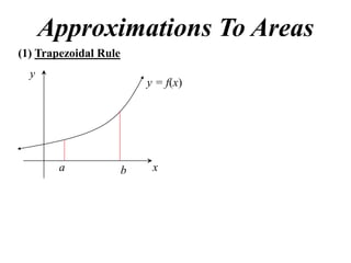
Slideshare is discontinuing its Slidecast feature as of February 28, 2014. Existing Slidecasts will be converted to static presentations without audio by April 30, 2014. The document informs users that new slidecasts can be found on myPlick.com or the author's blog starting in 2014. However, myPlick proved unreliable, so future slidecasts will instead be hosted on the author's YouTube channel.
The document discusses different methods for factorising expressions:
1) Looking for a common factor and dividing it out of all terms
2) Using the difference of two squares formula (a2 - b2 = (a - b)(a + b))
3) Factorising quadratic trinomials into two binomial factors by identifying the values that multiply to give the constant term and sum to give the coefficient of the linear term.
The document provides information on index laws and the meaning of indices in algebra:
- Index laws state that am × an = am+n, am ÷ an = am-n, and (am)n = amn. Exponents can be added or subtracted when multiplying or dividing terms with the same base.
- Positive exponents indicate a term is raised to a power. Negative exponents indicate a root is being taken. Terms with exponents are evaluated from left to right.
- Examples demonstrate how to simplify expressions using index laws and interpret different types of indices.
12 x1 t01 03 integrating derivative on function (2013)Nigel Simmons
The document discusses integrating derivatives of functions. It states that the integral of the derivative of a function f(x) is equal to the natural log of f(x) plus a constant. It then provides examples of integrating several derivatives: (i) ∫(1/(7-3x)) dx = -1/3 log(7-3x) + c, (ii) ∫(1/(8x+5)) dx = 1/8 log(8x+5) + c, and (iii) ∫(x5/(x-2)) dx = 1/6 log(x6-2) + c. It also discusses techniques for integrating fractions by polynomial long division and finds
The document discusses logarithms and their properties. Logarithms are defined as the inverse of exponentials. If y = ax, then x = loga y. The natural logarithm is log base e, written as ln. Properties of logarithms include: loga m + loga n = loga mn; loga m - loga n = loga(m/n); loga mn = n loga m; loga 1 = 0; loga a = 1. Examples of evaluating logarithmic expressions are provided.
The document discusses relationships between the coefficients and roots of polynomials. It states that for a polynomial P(x) = axn + bxn-1 + cxn-2 + ..., the sum of the roots equals -b/a, the sum of the roots taken two at a time equals c/a, and so on for higher order terms. It also provides examples of using these relationships to find the sums of roots for a given polynomial.
P
4
3
2
The document discusses properties of polynomials with multiple roots. It first proves that if a polynomial P(x) has a root x = a of multiplicity m, then the derivative of P(x), P'(x), will have a root x = a of multiplicity m-1. It then provides an example of solving a cubic equation given it has a double root. Finally, it examines a quartic polynomial and shows that its root α cannot be 0, 1, or -1, and that 1/
The document discusses factorizing complex expressions. The main points are:
- If a polynomial's coefficients are real, its roots will appear in complex conjugate pairs.
- Any polynomial of degree n can be factorized into a mixture of quadratic and linear factors over real numbers, or into n linear factors over complex numbers.
- Odd degree polynomials must have at least one real root.
- Examples of factorizing polynomials over both real and complex numbers are provided.
The document discusses nth roots of unity. It states that the solutions to equations of the form zn = ±1 are the nth roots of unity. These solutions form a regular n-sided polygon with vertices on the unit circle when placed on an Argand diagram. As an example, it shows that the solutions to z5 = 1 are the fifth roots of unity located at angles that are integer multiples of 2π/5 around the unit circle. It then proves that if ω is a root of z5 - 1 = 0, then ω2, ω3, ω4 and ω5 are also roots. Finally, it proves that 1 + ω + ω2 + ω3 + ω4 = 0.
The document discusses the geometric representation of complex numbers using vectors on the Argand diagram. It explains that complex numbers can be represented as vectors, with the real part of the number as the x-coordinate and imaginary part as the y-coordinate of the vector. Addition and subtraction of complex numbers corresponds to placing the vectors head to tail and head to head, respectively. Properties like the parallelogram law and triangle inequality are demonstrated. Multiplication of complex numbers is shown to be equivalent to multiplying the magnitudes and adding the arguments of the vectors.
How to Make a Field Mandatory in Odoo 17Celine George
In Odoo, making a field required can be done through both Python code and XML views. When you set the required attribute to True in Python code, it makes the field required across all views where it's used. Conversely, when you set the required attribute in XML views, it makes the field required only in the context of that particular view.
How to Add Chatter in the odoo 17 ERP ModuleCeline George
In Odoo, the chatter is like a chat tool that helps you work together on records. You can leave notes and track things, making it easier to talk with your team and partners. Inside chatter, all communication history, activity, and changes will be displayed.
This presentation was provided by Steph Pollock of The American Psychological Association’s Journals Program, and Damita Snow, of The American Society of Civil Engineers (ASCE), for the initial session of NISO's 2024 Training Series "DEIA in the Scholarly Landscape." Session One: 'Setting Expectations: a DEIA Primer,' was held June 6, 2024.
How to Build a Module in Odoo 17 Using the Scaffold MethodCeline George
Odoo provides an option for creating a module by using a single line command. By using this command the user can make a whole structure of a module. It is very easy for a beginner to make a module. There is no need to make each file manually. This slide will show how to create a module using the scaffold method.
A workshop hosted by the South African Journal of Science aimed at postgraduate students and early career researchers with little or no experience in writing and publishing journal articles.
हिंदी वर्णमाला पीपीटी, hindi alphabet PPT presentation, hindi varnamala PPT, Hindi Varnamala pdf, हिंदी स्वर, हिंदी व्यंजन, sikhiye hindi varnmala, dr. mulla adam ali, hindi language and literature, hindi alphabet with drawing, hindi alphabet pdf, hindi varnamala for childrens, hindi language, hindi varnamala practice for kids, https://www.drmullaadamali.com
How to Fix the Import Error in the Odoo 17Celine George
An import error occurs when a program fails to import a module or library, disrupting its execution. In languages like Python, this issue arises when the specified module cannot be found or accessed, hindering the program's functionality. Resolving import errors is crucial for maintaining smooth software operation and uninterrupted development processes.
Executive Directors Chat Leveraging AI for Diversity, Equity, and InclusionTechSoup
Let’s explore the intersection of technology and equity in the final session of our DEI series. Discover how AI tools, like ChatGPT, can be used to support and enhance your nonprofit's DEI initiatives. Participants will gain insights into practical AI applications and get tips for leveraging technology to advance their DEI goals.
ISO/IEC 27001, ISO/IEC 42001, and GDPR: Best Practices for Implementation and...PECB
Denis is a dynamic and results-driven Chief Information Officer (CIO) with a distinguished career spanning information systems analysis and technical project management. With a proven track record of spearheading the design and delivery of cutting-edge Information Management solutions, he has consistently elevated business operations, streamlined reporting functions, and maximized process efficiency.
Certified as an ISO/IEC 27001: Information Security Management Systems (ISMS) Lead Implementer, Data Protection Officer, and Cyber Risks Analyst, Denis brings a heightened focus on data security, privacy, and cyber resilience to every endeavor.
His expertise extends across a diverse spectrum of reporting, database, and web development applications, underpinned by an exceptional grasp of data storage and virtualization technologies. His proficiency in application testing, database administration, and data cleansing ensures seamless execution of complex projects.
What sets Denis apart is his comprehensive understanding of Business and Systems Analysis technologies, honed through involvement in all phases of the Software Development Lifecycle (SDLC). From meticulous requirements gathering to precise analysis, innovative design, rigorous development, thorough testing, and successful implementation, he has consistently delivered exceptional results.
Throughout his career, he has taken on multifaceted roles, from leading technical project management teams to owning solutions that drive operational excellence. His conscientious and proactive approach is unwavering, whether he is working independently or collaboratively within a team. His ability to connect with colleagues on a personal level underscores his commitment to fostering a harmonious and productive workplace environment.
Date: May 29, 2024
Tags: Information Security, ISO/IEC 27001, ISO/IEC 42001, Artificial Intelligence, GDPR
-------------------------------------------------------------------------------
Find out more about ISO training and certification services
Training: ISO/IEC 27001 Information Security Management System - EN | PECB
ISO/IEC 42001 Artificial Intelligence Management System - EN | PECB
General Data Protection Regulation (GDPR) - Training Courses - EN | PECB
Webinars: https://pecb.com/webinars
Article: https://pecb.com/article
-------------------------------------------------------------------------------
For more information about PECB:
Website: https://pecb.com/
LinkedIn: https://www.linkedin.com/company/pecb/
Facebook: https://www.facebook.com/PECBInternational/
Slideshare: http://www.slideshare.net/PECBCERTIFICATION
6. Approximations To Areas
(1) Trapezoidal Rule
y
y = f(x) ba
A f a f b
2
y y = f(x)
a b x
ca bc
A f a f c f c f b
2 2
a c b x
7. Approximations To Areas
(1) Trapezoidal Rule
y
y = f(x) ba
A f a f b
2
y y = f(x)
a b x
ca bc
A f a f c f c f b
2 2
ca
f a 2 f c f b
2
a c b x
10. y
y = f(x)
ca d c
A f a f c f c f d
2 2
bd
f d f b
2
a c d b x
11. y
y = f(x)
ca d c
A f a f c f c f d
2 2
bd
f d f b
2
a c d b x c a f a 2 f c 2 f d f b
2
12. y
y = f(x)
ca d c
A f a f c f c f d
2 2
bd
f d f b
2
a c d b x c a f a 2 f c 2 f d f b
2
In general;
13. y
y = f(x)
ca d c
A f a f c f c f d
2 2
bd
f d f b
2
a c d b x c a f a 2 f c 2 f d f b
2
In general; b
Area f x dx
a
14. y
y = f(x)
ca d c
A f a f c f c f d
2 2
bd
f d f b
2
a c d b x c a f a 2 f c 2 f d f b
2
In general; b
Area f x dx
a
h
y0 2 yothers yn
2
15. y
y = f(x)
ca d c
A f a f c f c f d
2 2
bd
f d f b
2
a c d b x c a f a 2 f c 2 f d f b
2
In general; b
Area f x dx
a
h
y0 2 yothers yn
2
ba
where h
n
n number of trapeziums
16. y
y = f(x)
ca d c
A f a f c f c f d
2 2
bd
f d f b
2
a c d b x c a f a 2 f c 2 f d f b
2
In general; b
Area f x dx
a
h
y0 2 yothers yn NOTE: there is
2
ba always one more
where h function value
n
than interval
n number of trapeziums
17. e.g. Use the Trapezoida l Rule with 4 intervals to estimate the
area under the curve y 4 x , between x 0 and x 2
1
2 2
correct to 3 decimal points
18. e.g. Use the Trapezoida l Rule with 4 intervals to estimate the
area under the curve y 4 x , between x 0 and x 2
1
2 2
correct to 3 decimal points
ba
h
n
20
4
0.5
19. e.g. Use the Trapezoida l Rule with 4 intervals to estimate the
area under the curve y 4 x , between x 0 and x 2
1
2 2
correct to 3 decimal points
ba
h
n x 0 0.5 1 1.5 2
20 y 2 1.9365 1.7321 1.3229 0
4
0.5
20. e.g. Use the Trapezoida l Rule with 4 intervals to estimate the
area under the curve y 4 x , between x 0 and x 2
1
2 2
correct to 3 decimal points
ba
h
n x 0 0.5 1 1.5 2
20 y 2 1.9365 1.7321 1.3229 0
h
4 Area y0 2 yothers yn
0.5 2
21. e.g. Use the Trapezoida l Rule with 4 intervals to estimate the
area under the curve y 4 x , between x 0 and x 2
1
2 2
correct to 3 decimal points
ba 1 1
h
n x 0 0.5 1 1.5 2
20 y 2 1.9365 1.7321 1.3229 0
h
4 Area y0 2 yothers yn
0.5 2
22. e.g. Use the Trapezoida l Rule with 4 intervals to estimate the
area under the curve y 4 x , between x 0 and x 2
1
2 2
correct to 3 decimal points
ba 1 2 2 2 1
h
n x 0 0.5 1 1.5 2
20 y 2 1.9365 1.7321 1.3229 0
h
4 Area y0 2 yothers yn
0.5 2
23. e.g. Use the Trapezoida l Rule with 4 intervals to estimate the
area under the curve y 4 x , between x 0 and x 2
1
2 2
correct to 3 decimal points
ba 1 2 2 2 1
h
n x 0 0.5 1 1.5 2
20 y 2 1.9365 1.7321 1.3229 0
h
4 Area y0 2 yothers yn
0.5 2
0.5
2 21.9365 1.7321 1.3229 0
2
2.996 units 2
24. e.g. Use the Trapezoida l Rule with 4 intervals to estimate the
area under the curve y 4 x , between x 0 and x 2
1
2 2
correct to 3 decimal points
ba 1 2 2 2 1
h
n x 0 0.5 1 1.5 2
20 y 2 1.9365 1.7321 1.3229 0
h
4 Area y0 2 yothers yn
0.5 2
0.5
2 21.9365 1.7321 1.3229 0
2
2.996 units 2 exact value π
25. e.g. Use the Trapezoida l Rule with 4 intervals to estimate the
area under the curve y 4 x , between x 0 and x 2
1
2 2
correct to 3 decimal points
ba 1 2 2 2 1
h
n x 0 0.5 1 1.5 2
20 y 2 1.9365 1.7321 1.3229 0
h
4 Area y0 2 yothers yn
0.5 2
0.5
2 21.9365 1.7321 1.3229 0
2
2.996 units 2 exact value π
3.142 2.996
% error 100
3.142
4.6%
28. (2) Simpson’s Rule
b
Area f x dx
a
h
y0 4 yodd 2 yeven yn
3
29. (2) Simpson’s Rule
b
Area f x dx
a
h
y0 4 yodd 2 yeven yn
3
ba
where h
n
n number of intervals
30. (2) Simpson’s Rule
b
Area f x dx
a
h
y0 4 yodd 2 yeven yn
3
ba
where h
n
n number of intervals
e.g.
x 0 0.5 1 1.5 2
y 2 1.9365 1.7321 1.3229 0
31. (2) Simpson’s Rule
b
Area f x dx
a
h
y0 4 yodd 2 yeven yn
3
ba
where h
n
n number of intervals
e.g.
x 0 0.5 1 1.5 2
y 2 1.9365 1.7321 1.3229 0
h
Area y0 4 yodd 2 yeven yn
3
32. (2) Simpson’s Rule
b
Area f x dx
a
h
y0 4 yodd 2 yeven yn
3
ba
where h
n
n number of intervals
e.g. 1 1
x 0 0.5 1 1.5 2
y 2 1.9365 1.7321 1.3229 0
h
Area y0 4 yodd 2 yeven yn
3
33. (2) Simpson’s Rule
b
Area f x dx
a
h
y0 4 yodd 2 yeven yn
3
ba
where h
n
n number of intervals
e.g. 1 4 4 1
x 0 0.5 1 1.5 2
y 2 1.9365 1.7321 1.3229 0
h
Area y0 4 yodd 2 yeven yn
3
34. (2) Simpson’s Rule
b
Area f x dx
a
h
y0 4 yodd 2 yeven yn
3
ba
where h
n
n number of intervals
e.g. 1 4 2 4 1
x 0 0.5 1 1.5 2
y 2 1.9365 1.7321 1.3229 0
h
Area y0 4 yodd 2 yeven yn
3
35. (2) Simpson’s Rule
b
Area f x dx
a
h
y0 4 yodd 2 yeven yn
3
ba
where h
n
n number of intervals
e.g. 1 4 2 4 1
x 0 0.5 1 1.5 2
y 2 1.9365 1.7321 1.3229 0
h
Area y0 4 yodd 2 yeven yn
3
0.5
2 41.9365 1.3229 21.7321 0
3
3.084 units 2
36. (2) Simpson’s Rule
b
Area f x dx
a
h
y0 4 yodd 2 yeven yn
3
ba
where h
n
n number of intervals
e.g. 1 4 2 4 1
x 0 0.5 1 1.5 2
y 2 1.9365 1.7321 1.3229 0
h
Area y0 4 yodd 2 yeven yn
3
0.5
2 41.9365 1.3229 21.7321 0 3.142 3.084
3 % error 100
3.084 units 2 3.142
1.8%