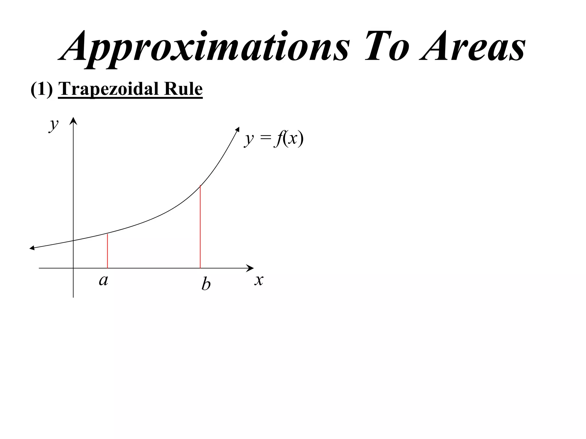
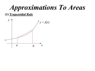
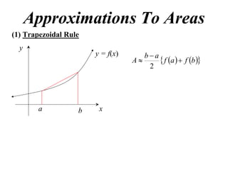
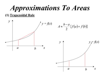
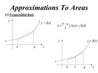
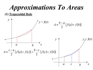
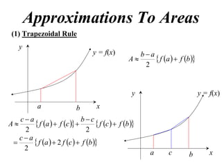
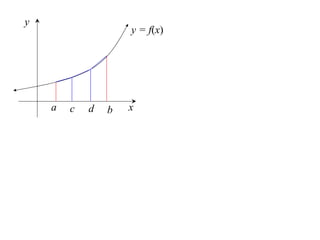
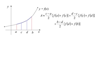
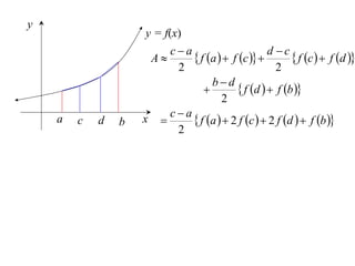
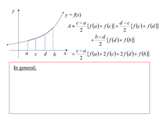
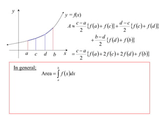
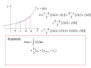
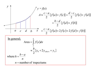
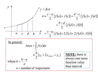
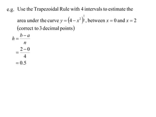
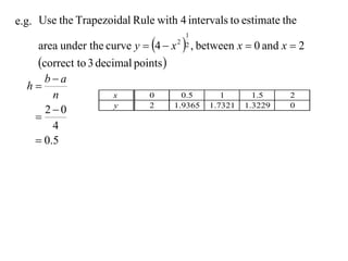
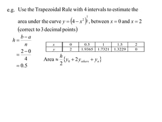
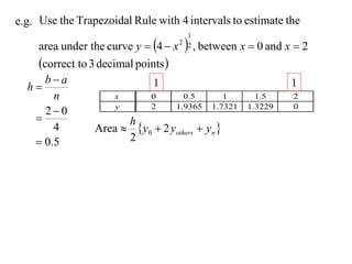
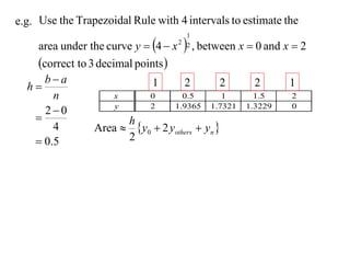
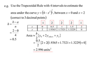
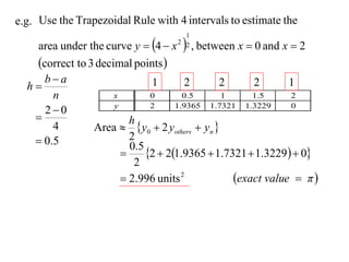
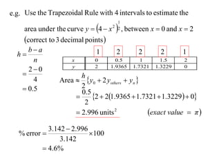
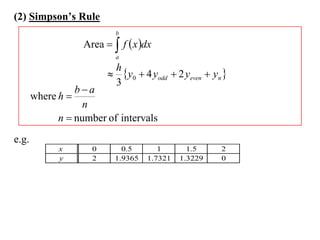
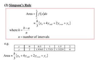
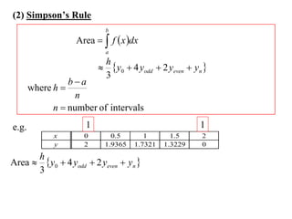
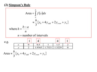
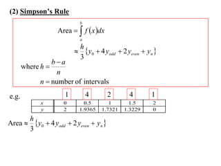
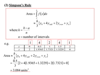
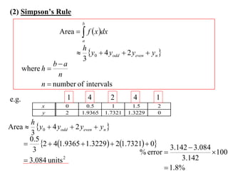
Approximations To Areas
(1) Trapezoidal Rule
  y
                       y = f(x)


       a           b    x
Approximations To Areas
(1) Trapezoidal Rule
  y
                       y = f(x)


       a           b    x
Approximations To Areas
(1) Trapezoidal Rule
  y
                       y = f(x)      ba
                                  A      f a   f b 
                                      2


       a           b    x
Approximations To Areas
(1) Trapezoidal Rule
  y
                       y = f(x)      ba
                                  A      f a   f b 
                                      2


                                   y                          y = f(x)
       a           b    x


                                          a             b         x
Approximations To Areas
(1) Trapezoidal Rule
  y
                       y = f(x)      ba
                                  A      f a   f b 
                                      2


                                   y                          y = f(x)
       a           b    x


                                          a     c       b         x
Approximations To Areas
(1) Trapezoidal Rule
     y
                                  y = f(x)          ba
                                                 A      f a   f b 
                                                     2


                                                  y                          y = f(x)
           a               b        x
     ca                      bc
A        f a   f c        f c   f b 
      2                        2


                                                         a     c       b         x
Approximations To Areas
(1) Trapezoidal Rule
     y
                                  y = f(x)          ba
                                                 A      f a   f b 
                                                     2


                                                  y                          y = f(x)
          a               b        x
  ca                      bc
A     f a   f c           f c   f b 
   2                          2
  ca
      f a   2 f c   f b 
   2
                                                         a     c       b         x
y
            y = f(x)


    a   b   x
y
                    y = f(x)


    a   c   d   b   x
y
                    y = f(x)
                           ca                      d c
                        A      f a   f c          f c   f d 
                            2                         2
                                    bd
                                           f d   f b 
                                       2
    a   c   d   b   x
y
                    y = f(x)
                        ca                        d c
                     A        f a   f c           f c   f d 
                          2                          2
                                   bd
                                          f d   f b 
                                      2
    a   c   d   b   x  c  a  f a   2 f c   2 f d   f b 
                          2
y
                      y = f(x)
                          ca                        d c
                       A        f a   f c           f c   f d 
                            2                          2
                                     bd
                                            f d   f b 
                                        2
     a    c   d   b   x  c  a  f a   2 f c   2 f d   f b 
                            2
In general;
y
                            y = f(x)
                                ca                        d c
                             A        f a   f c           f c   f d 
                                  2                          2
                                           bd
                                                  f d   f b 
                                              2
     a    c    d    b       x  c  a  f a   2 f c   2 f d   f b 
                                  2
In general;             b
              Area   f  x dx
                        a
                        h
                         y0  2 yothers  yn 
                        2
y
                              y = f(x)
                                  ca                        d c
                               A        f a   f c           f c   f d 
                                    2                          2
                                             bd
                                                    f d   f b 
                                                2
     a      c    d    b       x  c  a  f a   2 f c   2 f d   f b 
                                    2
In general;               b
                Area   f  x dx
                          a
                          h
                           y0  2 yothers  yn 
                          2
          ba
where h 
            n
      n  number of trapeziums
y
                              y = f(x)
                                  ca                        d c
                               A        f a   f c           f c   f d 
                                    2                          2
                                             bd
                                                    f d   f b 
                                                2
     a      c    d    b       x  c  a  f a   2 f c   2 f d   f b 
                                    2
In general;               b
                Area   f  x dx
                          a
                          h
                           y0  2 yothers  yn     NOTE: there is
                          2
          ba                                         always one more
where h                                              function value
            n
                                                      than interval
      n  number of trapeziums
e.g. Use the Trapezoidal Rule with 4 intervals to estimate the

     area under the curve y  4  x     , between x  0 and x  2
                                         1
                                       2 2


     correct to 3 decimal points 
e.g. Use the Trapezoidal Rule with 4 intervals to estimate the

   area under the curve y  4  x     , between x  0 and x  2
                                       1
                                     2 2


   correct to 3 decimal points 
     ba
  h
       n
     20
   
       4
    0.5
e.g. Use the Trapezoidal Rule with 4 intervals to estimate the

   area under the curve y  4  x  , between x  0 and x  2
                                     1
                                   2 2


   correct to 3 decimal points 
     ba
  h
       n             x      0       0.5     1     1.5      2
                     y
     20                    2     1.9365 1.7321 1.3229     0
   
       4
    0.5
e.g. Use the Trapezoidal Rule with 4 intervals to estimate the

   area under the curve y  4  x  , between x  0 and x  2
                                     1
                                   2 2


   correct to 3 decimal points 
     ba
  h
       n             x      0       0.5       1   1.5      2
                     y
     20                    2     1.9365 1.7321 1.3229     0
                      h
       4        Area  y0  2 yothers  yn 
    0.5               2
e.g. Use the Trapezoidal Rule with 4 intervals to estimate the

   area under the curve y  4  x  , between x  0 and x  2
                                     1
                                   2 2


   correct to 3 decimal points 
     ba                     1                            1
  h
       n             x      0       0.5       1   1.5      2
                     y
     20                    2     1.9365 1.7321 1.3229     0
                      h
       4        Area  y0  2 yothers  yn 
    0.5               2
e.g. Use the Trapezoidal Rule with 4 intervals to estimate the

   area under the curve y  4  x  , between x  0 and x  2
                                     1
                                   2 2


   correct to 3 decimal points 
     ba                     1      2        2     2      1
  h
       n             x      0       0.5       1   1.5      2
                     y
     20                    2     1.9365 1.7321 1.3229     0
                      h
       4        Area  y0  2 yothers  yn 
    0.5               2
e.g. Use the Trapezoidal Rule with 4 intervals to estimate the

   area under the curve y  4  x  , between x  0 and x  2
                                     1
                                   2 2


   correct to 3 decimal points 
     ba                      1       2       2      2      1
  h
       n             x        0       0.5     1      1.5     2
                     y
     20                      2     1.9365 1.7321 1.3229     0
                        h
       4        Area  y0  2 yothers  yn 
    0.5                 2
                         0.5
                            2  21.9365  1.7321  1.3229  0
                          2
                        2.996 units 2
e.g. Use the Trapezoidal Rule with 4 intervals to estimate the

   area under the curve y  4  x  , between x  0 and x  2
                                     1
                                   2 2


   correct to 3 decimal points 
     ba                      1       2       2      2       1
  h
       n             x        0       0.5     1      1.5     2
                     y
     20                      2     1.9365 1.7321 1.3229     0
                        h
       4        Area  y0  2 yothers  yn 
    0.5                 2
                         0.5
                            2  21.9365  1.7321  1.3229  0
                          2
                        2.996 units 2           exact value  π 
             3.142  2.996
   % error                100
                 3.142
            4.6%
(2) Simpson’s Rule
(2) Simpson’s Rule
                      b
              Area   f  x dx
                      a
(2) Simpson’s Rule
                       b
              Area   f  x dx
                       a
                      h
                      y0  4 yodd  2 yeven  yn 
                      3
(2) Simpson’s Rule
                       b
               Area   f  x dx
                       a
                      h
                      y0  4 yodd  2 yeven  yn 
                      3
             ba
   where h 
               n
         n  number of intervals
(2) Simpson’s Rule
                           b
                   Area   f  x dx
                           a
                          h
                          y0  4 yodd  2 yeven  yn 
                          3
                 ba
       where h 
                   n
             n  number of intervals
e.g.
             x       0       0.5       1       1.5    2
             y       2     1.9365   1.7321   1.3229   0
(2) Simpson’s Rule
                             b
                    Area   f  x dx
                             a
                           h
                           y0  4 yodd  2 yeven  yn 
                           3
                 ba
       where h 
                   n
             n  number of intervals
e.g.
             x        0       0.5       1       1.5    2
             y        2     1.9365   1.7321   1.3229   0
         h
Area      y0  4 yodd  2 yeven  yn 
         3
(2) Simpson’s Rule
                             b
                    Area   f  x dx
                             a
                            h
                            y0  4 yodd  2 yeven  yn 
                            3
                 ba
       where h 
                   n
             n  number of intervals
e.g.                   1                                1
             x        0       0.5       1       1.5     2
             y        2     1.9365   1.7321   1.3229    0
         h
Area      y0  4 yodd  2 yeven  yn 
         3
(2) Simpson’s Rule
                             b
                    Area   f  x dx
                             a
                            h
                            y0  4 yodd  2 yeven  yn 
                            3
                 ba
       where h 
                   n
             n  number of intervals
e.g.                   1         4             4        1
             x        0       0.5       1       1.5     2
             y        2     1.9365   1.7321   1.3229    0
         h
Area      y0  4 yodd  2 yeven  yn 
         3
(2) Simpson’s Rule
                             b
                    Area   f  x dx
                             a
                            h
                            y0  4 yodd  2 yeven  yn 
                            3
                 ba
       where h 
                   n
             n  number of intervals
e.g.                   1         4         2    4       1
             x        0       0.5       1        1.5    2
             y        2     1.9365   1.7321    1.3229   0
         h
Area      y0  4 yodd  2 yeven  yn 
         3
(2) Simpson’s Rule
                           b
                   Area   f  x dx
                           a
                          h
                          y0  4 yodd  2 yeven  yn 
                          3
                 ba
       where h 
                   n
             n  number of intervals
e.g.                 1         4        2     4       1
             x       0       0.5       1       1.5      2
             y       2     1.9365   1.7321   1.3229     0
         h
Area      y0  4 yodd  2 yeven  yn 
         3
         0.5
            2  41.9365  1.3229  21.7321  0
          3
        3.084 units 2
(2) Simpson’s Rule
                           b
                   Area   f  x dx
                           a
                          h
                          y0  4 yodd  2 yeven  yn 
                          3
                 ba
       where h 
                   n
             n  number of intervals
e.g.                 1         4        2     4       1
             x       0       0.5       1       1.5    2
             y       2     1.9365   1.7321   1.3229   0
         h
Area      y0  4 yodd  2 yeven  yn 
         3
         0.5
            2  41.9365  1.3229  21.7321  0 3.142  3.084
          3                                   % error              100
        3.084 units 2                                      3.142
                                                       1.8%
Exercise 11I; odds

Exercise 11J; evens

11X1 T14 07 approximations

  • 1.
    Approximations To Areas (1)Trapezoidal Rule y y = f(x) a b x
  • 2.
    Approximations To Areas (1)Trapezoidal Rule y y = f(x) a b x
  • 3.
    Approximations To Areas (1)Trapezoidal Rule y y = f(x) ba A  f a   f b  2 a b x
  • 4.
    Approximations To Areas (1)Trapezoidal Rule y y = f(x) ba A  f a   f b  2 y y = f(x) a b x a b x
  • 5.
    Approximations To Areas (1)Trapezoidal Rule y y = f(x) ba A  f a   f b  2 y y = f(x) a b x a c b x
  • 6.
    Approximations To Areas (1)Trapezoidal Rule y y = f(x) ba A  f a   f b  2 y y = f(x) a b x ca bc A  f a   f c    f c   f b  2 2 a c b x
  • 7.
    Approximations To Areas (1)Trapezoidal Rule y y = f(x) ba A  f a   f b  2 y y = f(x) a b x ca bc A  f a   f c    f c   f b  2 2 ca   f a   2 f c   f b  2 a c b x
  • 8.
    y y = f(x) a b x
  • 9.
    y y = f(x) a c d b x
  • 10.
    y y = f(x) ca d c A  f a   f c    f c   f d  2 2 bd   f d   f b  2 a c d b x
  • 11.
    y y = f(x) ca d c A  f a   f c    f c   f d  2 2 bd   f d   f b  2 a c d b x  c  a  f a   2 f c   2 f d   f b  2
  • 12.
    y y = f(x) ca d c A  f a   f c    f c   f d  2 2 bd   f d   f b  2 a c d b x  c  a  f a   2 f c   2 f d   f b  2 In general;
  • 13.
    y y = f(x) ca d c A  f a   f c    f c   f d  2 2 bd   f d   f b  2 a c d b x  c  a  f a   2 f c   2 f d   f b  2 In general; b Area   f  x dx a
  • 14.
    y y = f(x) ca d c A  f a   f c    f c   f d  2 2 bd   f d   f b  2 a c d b x  c  a  f a   2 f c   2 f d   f b  2 In general; b Area   f  x dx a h  y0  2 yothers  yn  2
  • 15.
    y y = f(x) ca d c A  f a   f c    f c   f d  2 2 bd   f d   f b  2 a c d b x  c  a  f a   2 f c   2 f d   f b  2 In general; b Area   f  x dx a h  y0  2 yothers  yn  2 ba where h  n n  number of trapeziums
  • 16.
    y y = f(x) ca d c A  f a   f c    f c   f d  2 2 bd   f d   f b  2 a c d b x  c  a  f a   2 f c   2 f d   f b  2 In general; b Area   f  x dx a h  y0  2 yothers  yn  NOTE: there is 2 ba always one more where h  function value n than interval n  number of trapeziums
  • 17.
    e.g. Use theTrapezoidal Rule with 4 intervals to estimate the area under the curve y  4  x  , between x  0 and x  2 1 2 2 correct to 3 decimal points 
  • 18.
    e.g. Use theTrapezoidal Rule with 4 intervals to estimate the area under the curve y  4  x  , between x  0 and x  2 1 2 2 correct to 3 decimal points  ba h n 20  4  0.5
  • 19.
    e.g. Use theTrapezoidal Rule with 4 intervals to estimate the area under the curve y  4  x  , between x  0 and x  2 1 2 2 correct to 3 decimal points  ba h n x 0 0.5 1 1.5 2 y 20 2 1.9365 1.7321 1.3229 0  4  0.5
  • 20.
    e.g. Use theTrapezoidal Rule with 4 intervals to estimate the area under the curve y  4  x  , between x  0 and x  2 1 2 2 correct to 3 decimal points  ba h n x 0 0.5 1 1.5 2 y 20 2 1.9365 1.7321 1.3229 0  h 4 Area  y0  2 yothers  yn   0.5 2
  • 21.
    e.g. Use theTrapezoidal Rule with 4 intervals to estimate the area under the curve y  4  x  , between x  0 and x  2 1 2 2 correct to 3 decimal points  ba 1 1 h n x 0 0.5 1 1.5 2 y 20 2 1.9365 1.7321 1.3229 0  h 4 Area  y0  2 yothers  yn   0.5 2
  • 22.
    e.g. Use theTrapezoidal Rule with 4 intervals to estimate the area under the curve y  4  x  , between x  0 and x  2 1 2 2 correct to 3 decimal points  ba 1 2 2 2 1 h n x 0 0.5 1 1.5 2 y 20 2 1.9365 1.7321 1.3229 0  h 4 Area  y0  2 yothers  yn   0.5 2
  • 23.
    e.g. Use theTrapezoidal Rule with 4 intervals to estimate the area under the curve y  4  x  , between x  0 and x  2 1 2 2 correct to 3 decimal points  ba 1 2 2 2 1 h n x 0 0.5 1 1.5 2 y 20 2 1.9365 1.7321 1.3229 0  h 4 Area  y0  2 yothers  yn   0.5 2 0.5  2  21.9365  1.7321  1.3229  0 2  2.996 units 2
  • 24.
    e.g. Use theTrapezoidal Rule with 4 intervals to estimate the area under the curve y  4  x  , between x  0 and x  2 1 2 2 correct to 3 decimal points  ba 1 2 2 2 1 h n x 0 0.5 1 1.5 2 y 20 2 1.9365 1.7321 1.3229 0  h 4 Area  y0  2 yothers  yn   0.5 2 0.5  2  21.9365  1.7321  1.3229  0 2  2.996 units 2 exact value  π 
  • 25.
    e.g. Use theTrapezoidal Rule with 4 intervals to estimate the area under the curve y  4  x  , between x  0 and x  2 1 2 2 correct to 3 decimal points  ba 1 2 2 2 1 h n x 0 0.5 1 1.5 2 y 20 2 1.9365 1.7321 1.3229 0  h 4 Area  y0  2 yothers  yn   0.5 2 0.5  2  21.9365  1.7321  1.3229  0 2  2.996 units 2 exact value  π  3.142  2.996 % error  100 3.142  4.6%
  • 26.
  • 27.
    (2) Simpson’s Rule b Area   f  x dx a
  • 28.
    (2) Simpson’s Rule b Area   f  x dx a h  y0  4 yodd  2 yeven  yn  3
  • 29.
    (2) Simpson’s Rule b Area   f  x dx a h  y0  4 yodd  2 yeven  yn  3 ba where h  n n  number of intervals
  • 30.
    (2) Simpson’s Rule b Area   f  x dx a h  y0  4 yodd  2 yeven  yn  3 ba where h  n n  number of intervals e.g. x 0 0.5 1 1.5 2 y 2 1.9365 1.7321 1.3229 0
  • 31.
    (2) Simpson’s Rule b Area   f  x dx a h  y0  4 yodd  2 yeven  yn  3 ba where h  n n  number of intervals e.g. x 0 0.5 1 1.5 2 y 2 1.9365 1.7321 1.3229 0 h Area  y0  4 yodd  2 yeven  yn  3
  • 32.
    (2) Simpson’s Rule b Area   f  x dx a h  y0  4 yodd  2 yeven  yn  3 ba where h  n n  number of intervals e.g. 1 1 x 0 0.5 1 1.5 2 y 2 1.9365 1.7321 1.3229 0 h Area  y0  4 yodd  2 yeven  yn  3
  • 33.
    (2) Simpson’s Rule b Area   f  x dx a h  y0  4 yodd  2 yeven  yn  3 ba where h  n n  number of intervals e.g. 1 4 4 1 x 0 0.5 1 1.5 2 y 2 1.9365 1.7321 1.3229 0 h Area  y0  4 yodd  2 yeven  yn  3
  • 34.
    (2) Simpson’s Rule b Area   f  x dx a h  y0  4 yodd  2 yeven  yn  3 ba where h  n n  number of intervals e.g. 1 4 2 4 1 x 0 0.5 1 1.5 2 y 2 1.9365 1.7321 1.3229 0 h Area  y0  4 yodd  2 yeven  yn  3
  • 35.
    (2) Simpson’s Rule b Area   f  x dx a h  y0  4 yodd  2 yeven  yn  3 ba where h  n n  number of intervals e.g. 1 4 2 4 1 x 0 0.5 1 1.5 2 y 2 1.9365 1.7321 1.3229 0 h Area  y0  4 yodd  2 yeven  yn  3 0.5  2  41.9365  1.3229  21.7321  0 3  3.084 units 2
  • 36.
    (2) Simpson’s Rule b Area   f  x dx a h  y0  4 yodd  2 yeven  yn  3 ba where h  n n  number of intervals e.g. 1 4 2 4 1 x 0 0.5 1 1.5 2 y 2 1.9365 1.7321 1.3229 0 h Area  y0  4 yodd  2 yeven  yn  3 0.5  2  41.9365  1.3229  21.7321  0 3.142  3.084 3 % error  100  3.084 units 2 3.142  1.8%
  • 37.