Download to read offline

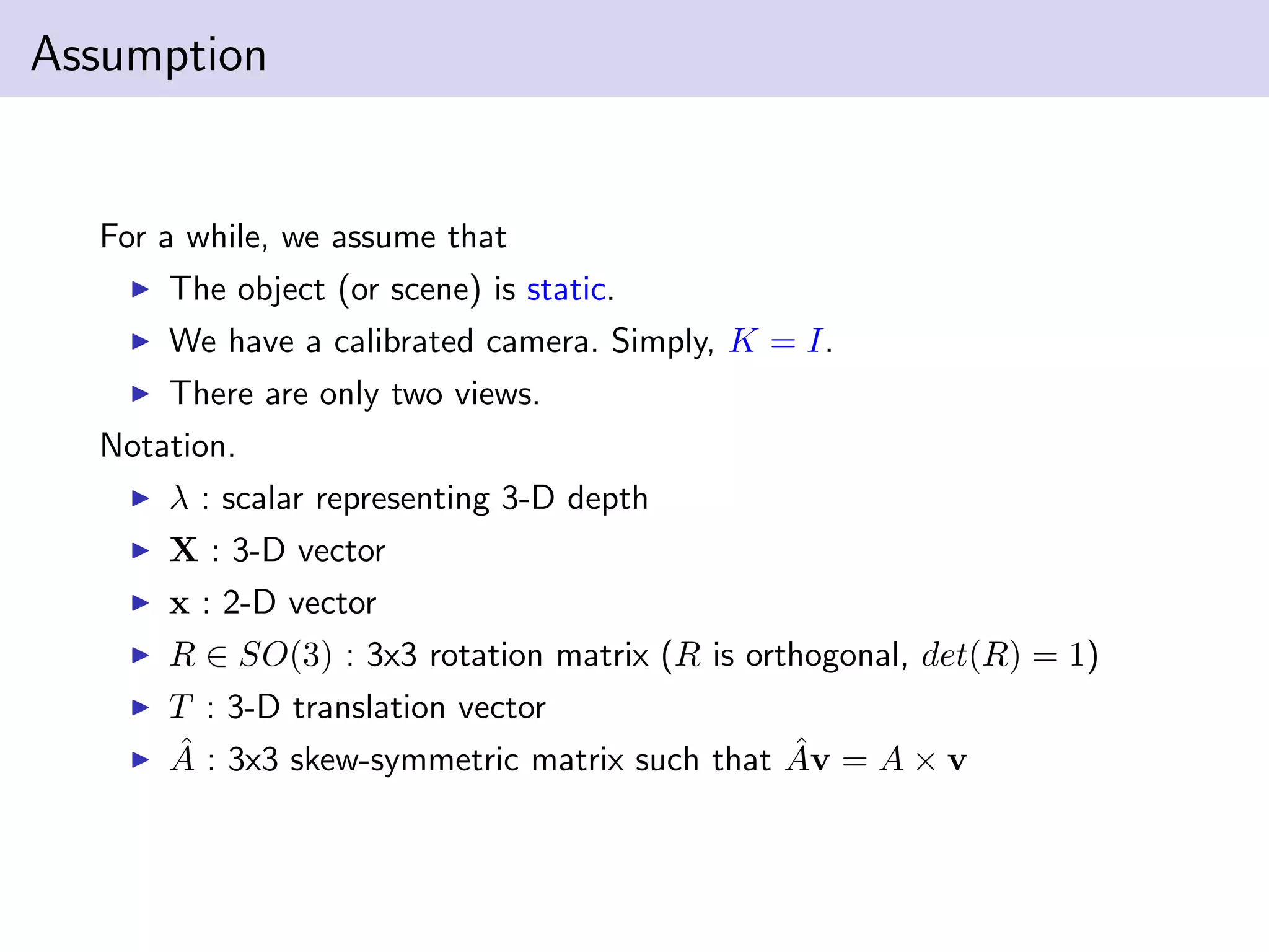
![Kronecker product and stack of matries
The following is useful when A is the only unknown.
xT
2 Ax1 = 0 ⇐⇒ (x1 ⊗ x2)T
As
= 0
(We saw this in the conjugate gradient lecture. x2 and x1 are
A-orthogonal or conjugate.)
x1⊗x2 = a = [x1x2, x1y2, x1z2, y1x2, y1y2, y1z2, z1x2, z1y2, z1z2]T
∈ R9
.
(Kronecker product)
Kronecker product of two vectors is also a vector.
We can stack elements of a matrix column-wise.
Es
= [e11, e21, e31, e12, e22, e23, e13, e23, e33]T
∈ R9
.
(stack of a matrix E)
A stack of a matrix is a vector.](https://image.slidesharecdn.com/journey-structure-motion-2-180419102403/75/Journey-to-structure-from-motion-25-2048.jpg)
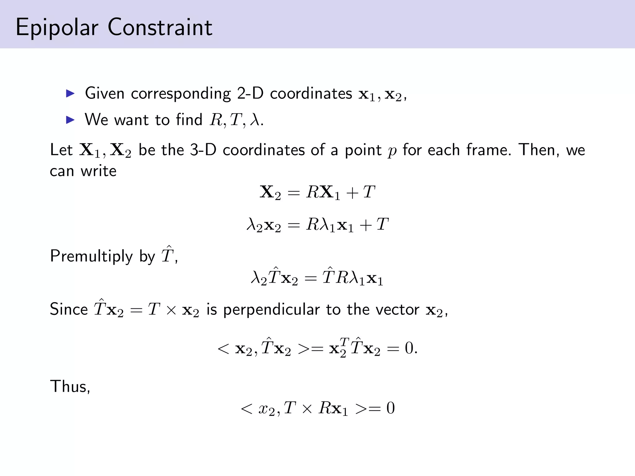
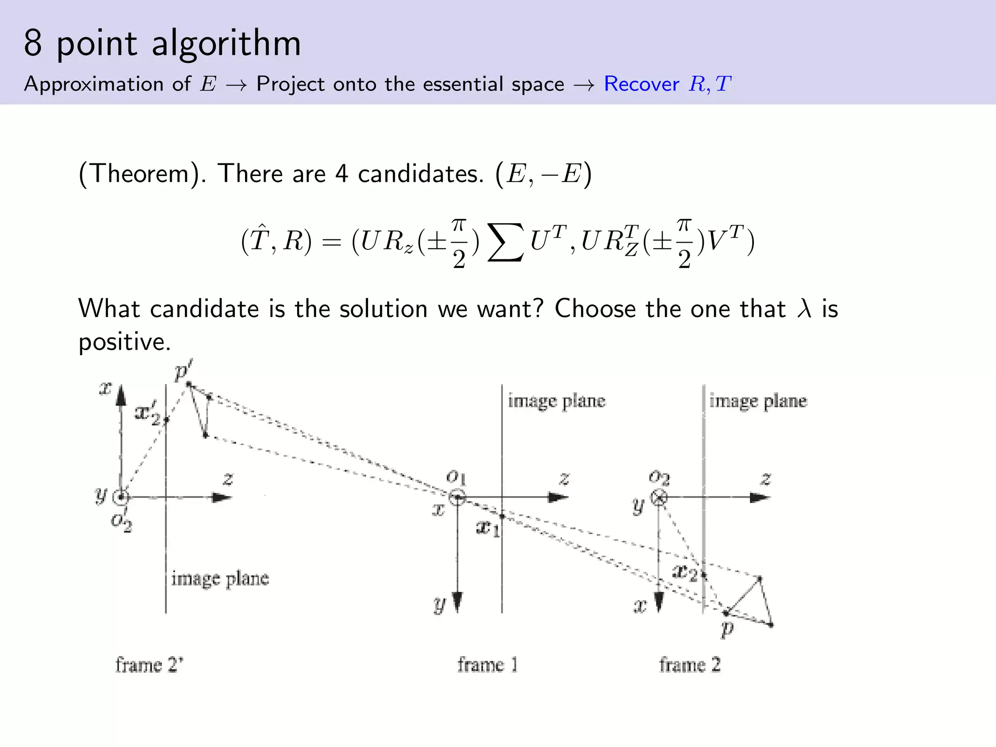
![8 point algorithm
Approximation of E → Project onto the essential space → Recover R, T
Idea : Decompose known and unknown, approximate E and then recover
R, T.
input : n image correspondences (xj
1, xj
2), j = 1, 2, ..., n(n ≥ 8)
From the input data, we can set
χ = [a1
, a2
, · · · , an
]T
∈ Rn∗9
where aj
= xj
1 ⊗ xj
2 ∈ R9
. From the epipolar constraint xT
2
ˆTRx1 = 0,
we can rewrite
χEs
= 0.
(Rank theorem) When A is m-by-n matrix,
rank(A) + dimNul(A) = n
If rank(χ) = 8,
rank(χ) + dimNul(χ) = 8 + dimNul(χ) = 9.
Then, we can get Es
up to scale. So we need at least 8 points.](https://image.slidesharecdn.com/journey-structure-motion-2-180419102403/75/Journey-to-structure-from-motion-26-2048.jpg)
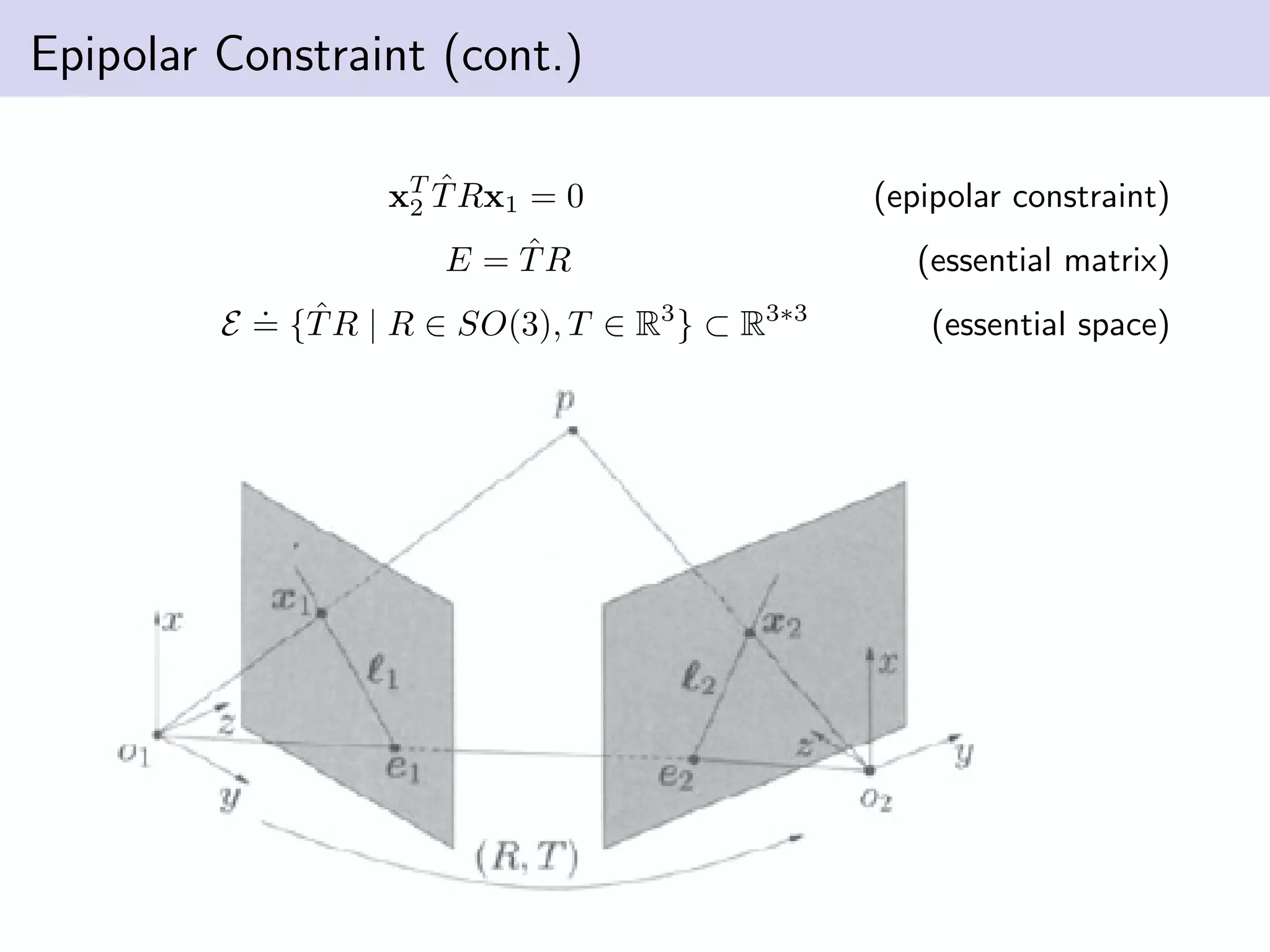
![8 point algorithm
Approximation of E → Project onto the essential space → Recover R, T
Theorem. E is an essential matrix if and only if
E = UΣV T
such that Σ = diag{σ, σ, 0}
where σ > 0 and U, V ∈ SO(3).
So we just have to replace the singular values with 1, 1.
% c o n s t r u c t chi matrix
chi = zeros (n , 9 ) ;
f o r i =1:n
chi ( i , : ) = kron ( [ featx1 ( i ) ; featy1 ( i ) ; 1 ] , [ featx2 ( i ) ;
end
% f i n d E stakced that minimizes | chi ∗ E stacked |
[ U chi , S chi , V chi ] = svd ( chi ) ;
E stacked = V chi ( : , 9 ) ;
% Pro jec t E onto e s s e n t i a l space
S (1 ,1) = 1; S (2 ,2) = 1; S (3 ,3) = 0;
% Get e s s e n t i a l matrix](https://image.slidesharecdn.com/journey-structure-motion-2-180419102403/75/Journey-to-structure-from-motion-28-2048.jpg)
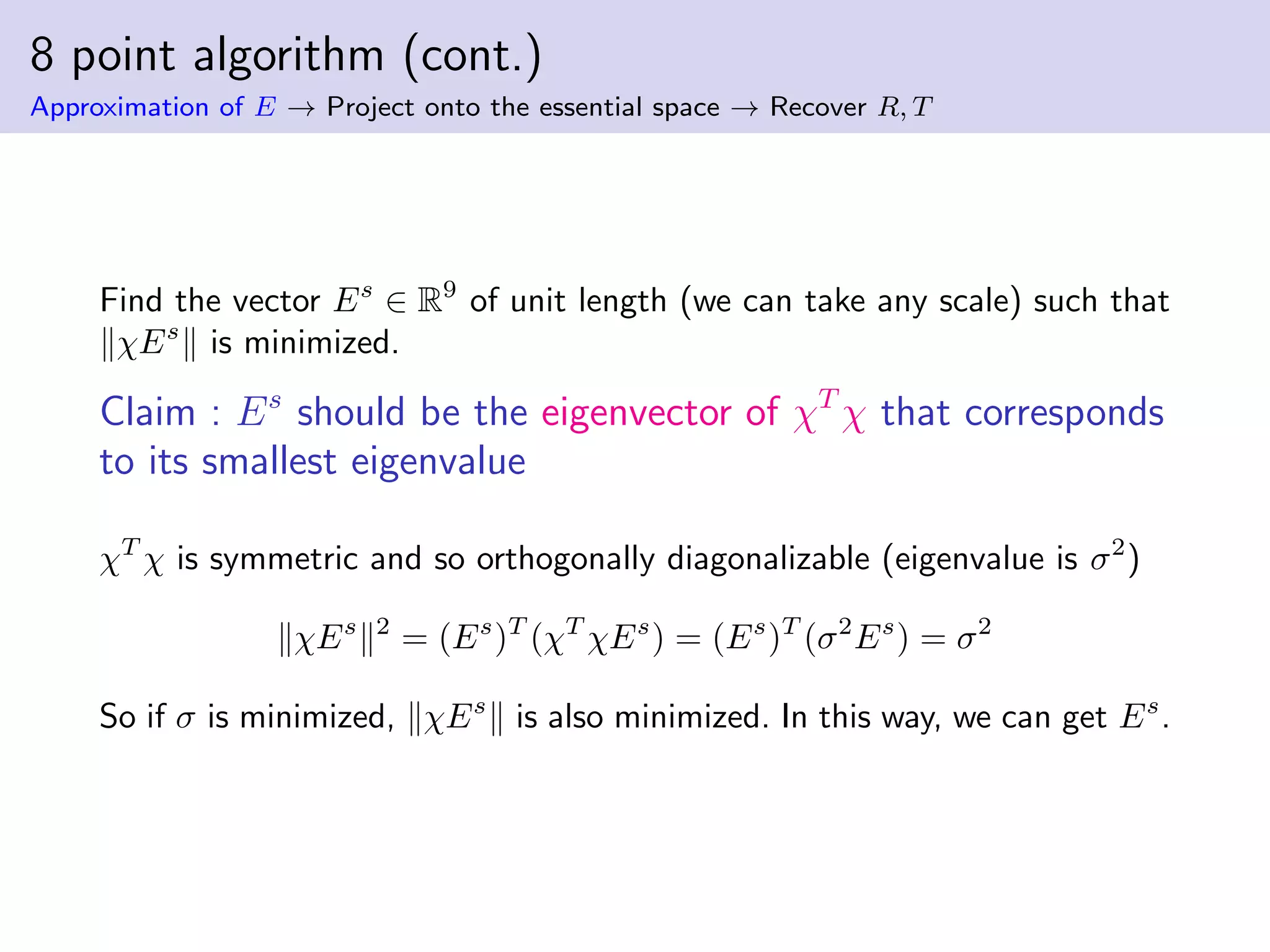
![Reconstruction from Two Calibrated Views
Approximation of E → Project onto the essential space → Recover R, T → Reconstruction
λj
2xj
2 = λj
1Rxj
1 + γT, j = 1, 2, ..., n
To reduce λ2, multiplying both sides by xj
2, we can get
0 = λj
1xj
2Rxj
1 + γxj
2T
Decompose known and unknown
Mj
λj .
= xj
2Rxj
1 xj
2T
λj
1
γ
= 0 (1)
Moreover, we can set
v = [λ1
1, λ2
1, ..., λn
1 , γ]T
∈ Rn+1
M =
ˆx1
2Rx1
1 0 0 ... ˆx1
2T
0 ˆx2
2Rx2
1 0 ... ...
0 0 ... ˆxn
2 Rxn
1 ˆxn
2 T
Mv = 0
The linear least-squares estimate of v is simply the eigenvector of MT
M
that corresponds to its smallest eigenvalue.](https://image.slidesharecdn.com/journey-structure-motion-2-180419102403/75/Journey-to-structure-from-motion-30-2048.jpg)
![Motion Estimation from Known Structure
Assume we have the depth of the points and thus their inverse αj
(i.e.
known structure). Then the above equation is linear in the camera motion
parameters Ri and Ti. Using the stack notation i = 2, 3, ..., m (fixed)
Pi
Rs
i
Ti
.
=
x1
1
T
⊗ x1
i α1
x1
i
x2
1
T
⊗ x2
i α2
x2
i
... ...
xn
1
T
⊗ xn
i αn
xn
i
Rs
i
Ti
= 0, ∈ R3n
It can be shown that if the αj
’s are known, the matrix Pi ∈ R3n×12
is of
rank 11 if more than n ≥ 6 points in general position are given. In that
case, the null space of Pi is unique up to a scale factor, and so is the
projection matrix Πi = [Ri, Ti]. (each of three (3n) are linearly
independent).
This does not decouple the structure and motion, completely. Firstly,
structure information is needed.](https://image.slidesharecdn.com/journey-structure-motion-2-180419102403/75/Journey-to-structure-from-motion-37-2048.jpg)

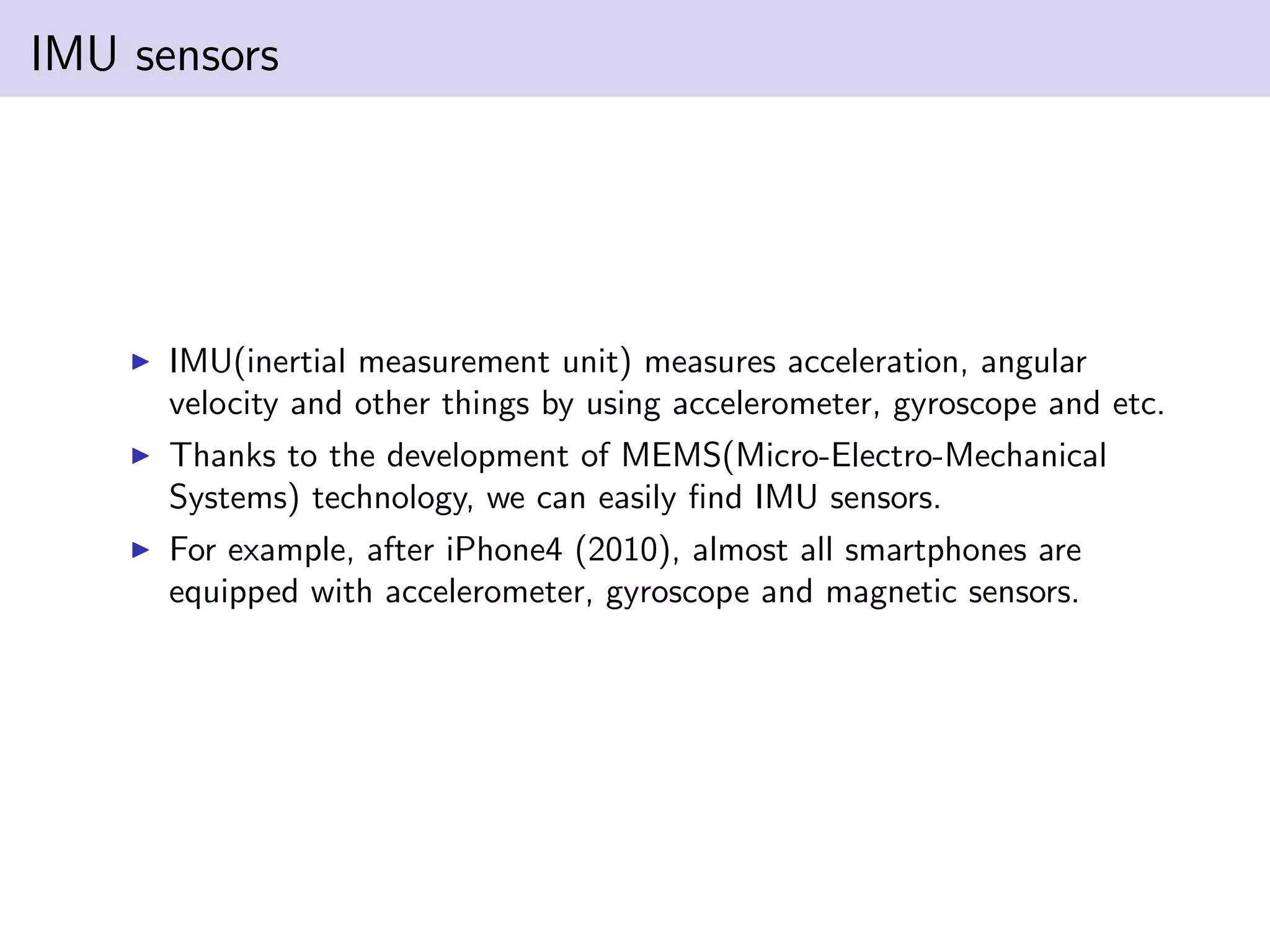
![Biological Motivation: Human Inertial Sensors
The utricle measures acceleration in the horizontal direction and the
saccule measures in the vertical direction.
The semicircular canals detect angular velocity of the head and are
oriented in three orthogonal planes. [1]
http://www.nebraskamed.com/health-library/
3d-medical-atlas/302/balance-and-equilibrium](https://image.slidesharecdn.com/journey-structure-motion-2-180419102403/75/Journey-to-structure-from-motion-43-2048.jpg)
![KLT tracker with IMU
We want to understand, implement and test by using our data.
Hwangbo, Kim, and Kanade, 2009 “Inertial-Aided KLT Feature Tracking
for a Moving Camera.” [2]
https://www.youtube.com/watch?v=a81WzJONPGA](https://image.slidesharecdn.com/journey-structure-motion-2-180419102403/75/Journey-to-structure-from-motion-46-2048.jpg)
![References
[1] P. Corke, J. Lobo, and J. Dias. An Introduction to Inertial and Visual
Sensing. The International Journal of Robotics Research,
26(6):519–535, June 2007.
[2] Myung Hwangbo, Jun-Sik Kim, and Takeo Kanade. Inertial-aided
KLT feature tracking for a moving camera. In Intelligent Robots and
Systems, 2009. IROS 2009. IEEE/RSJ International Conference on,
pages 1909–1916. IEEE.](https://image.slidesharecdn.com/journey-structure-motion-2-180419102403/75/Journey-to-structure-from-motion-55-2048.jpg)

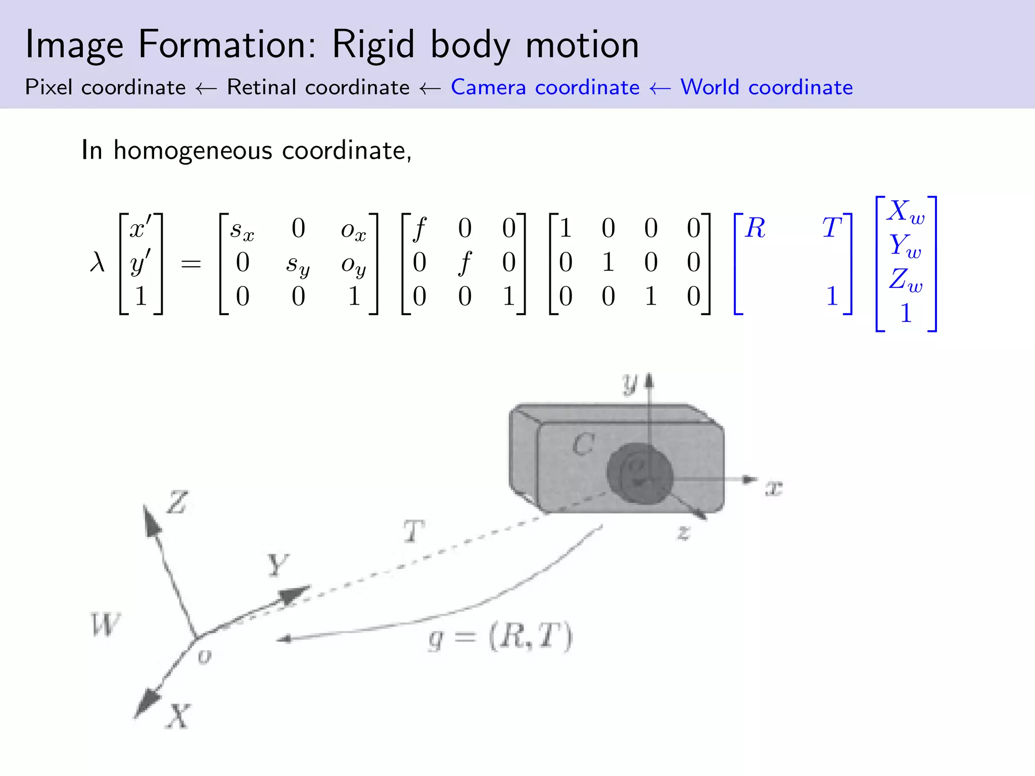
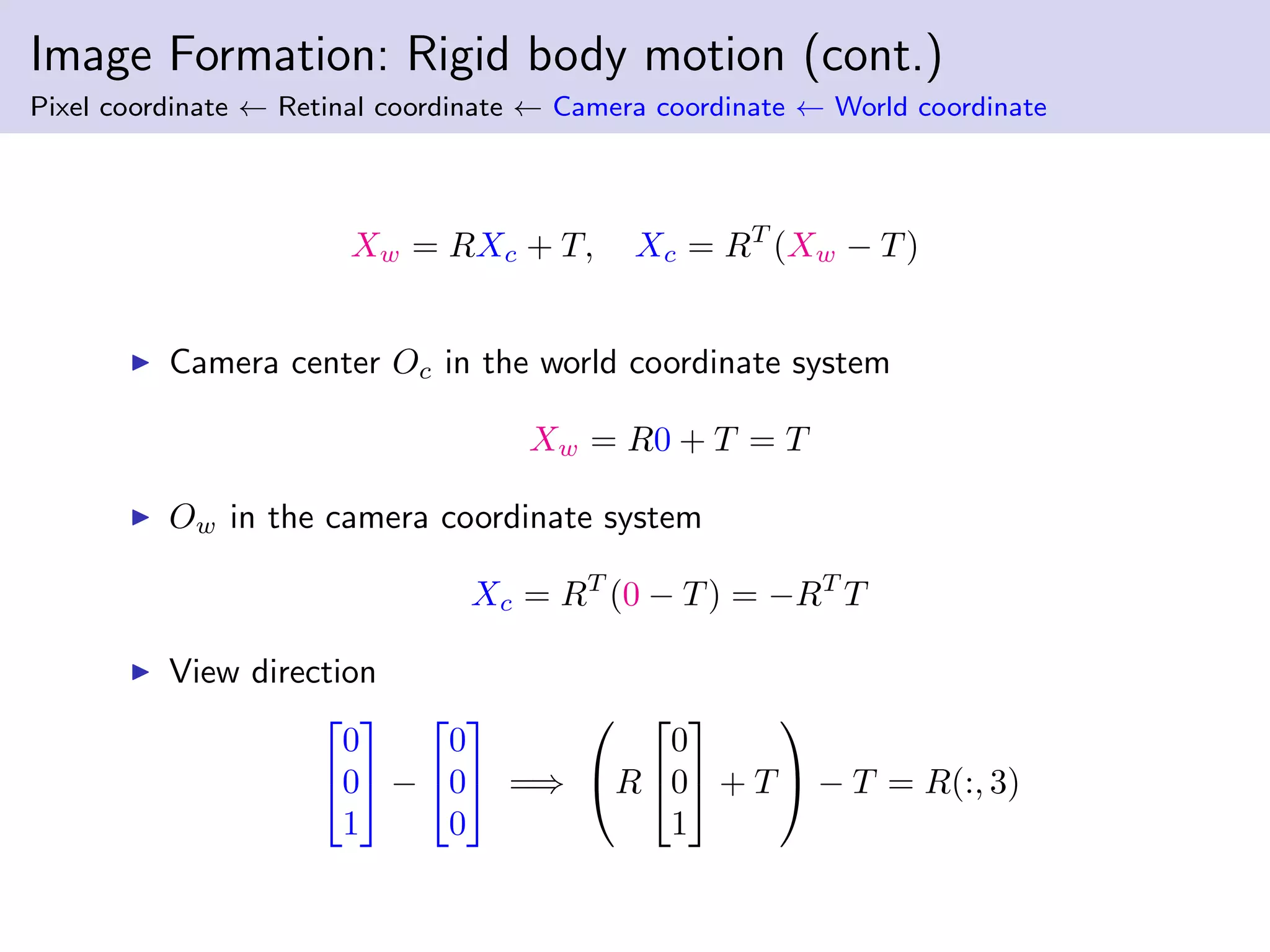
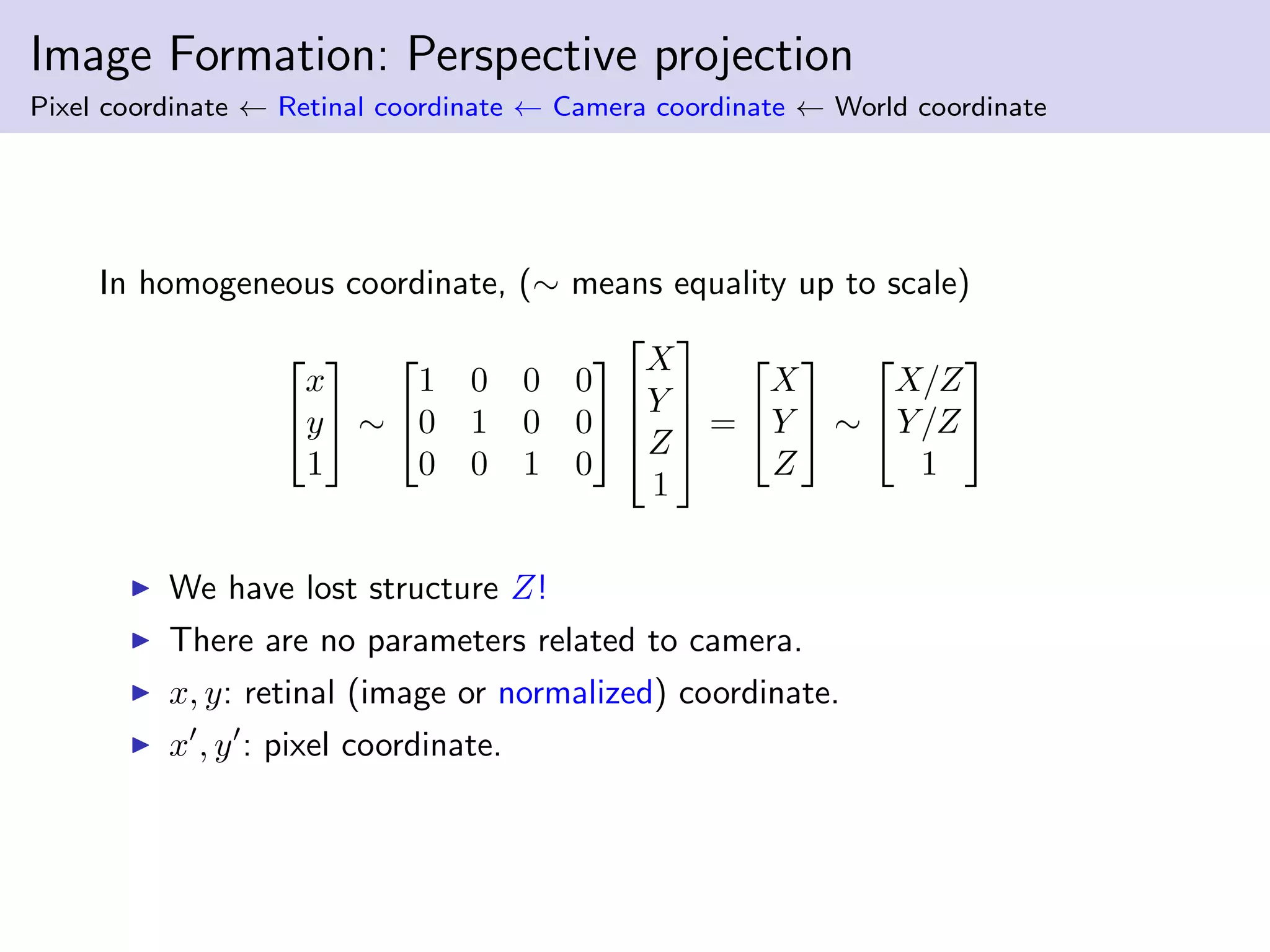
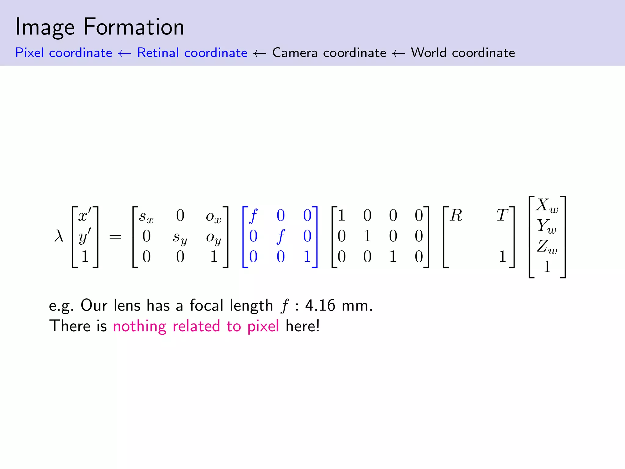
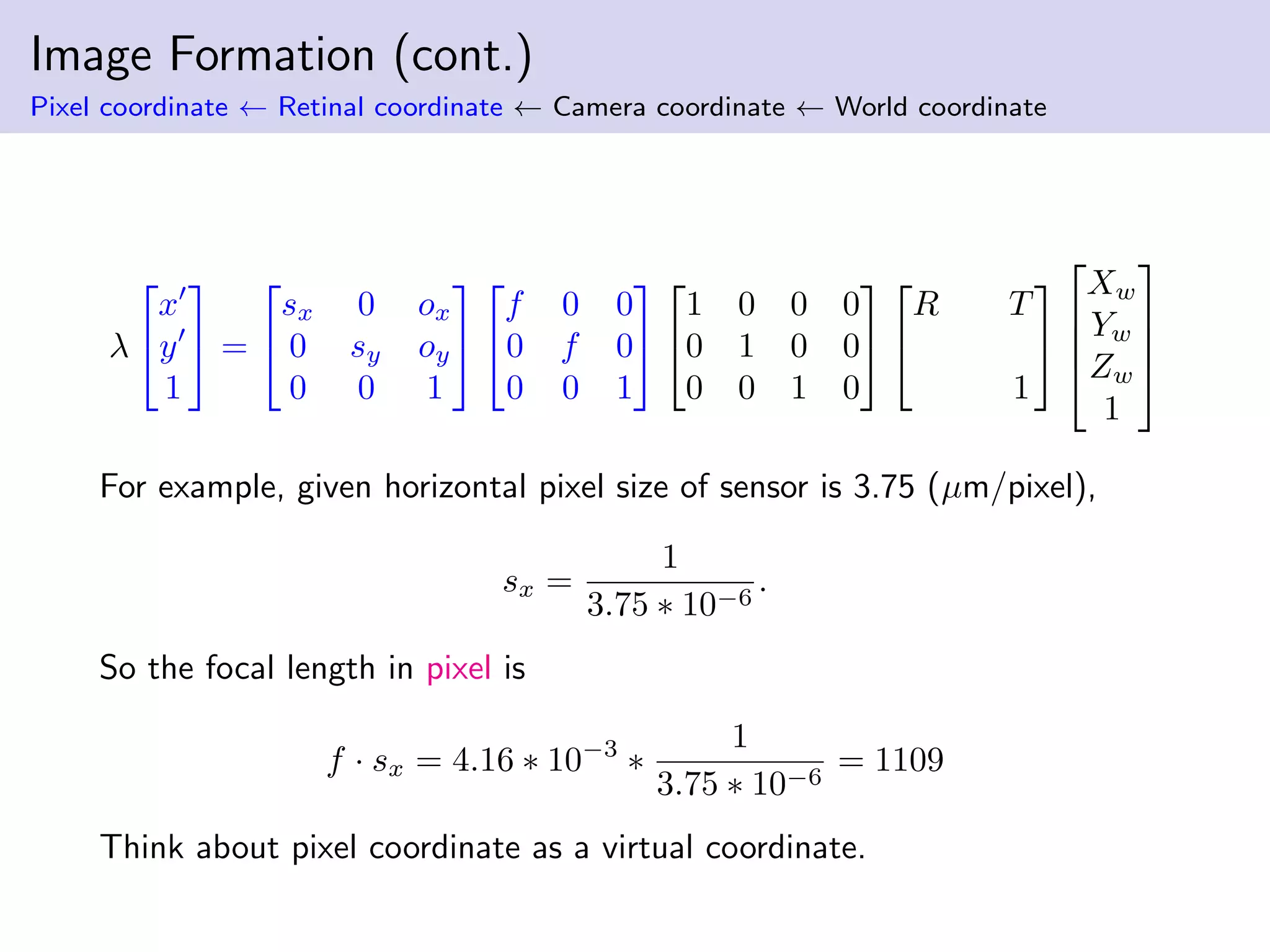
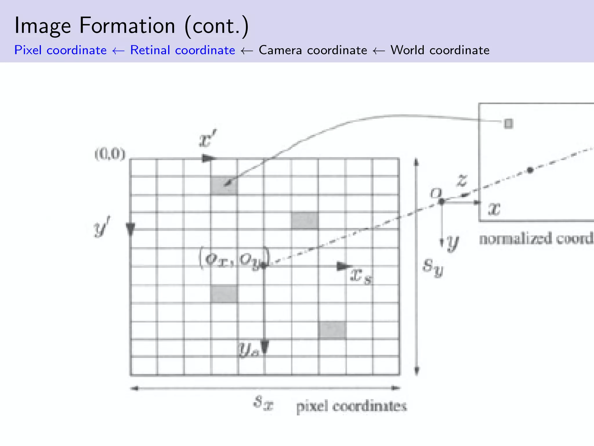
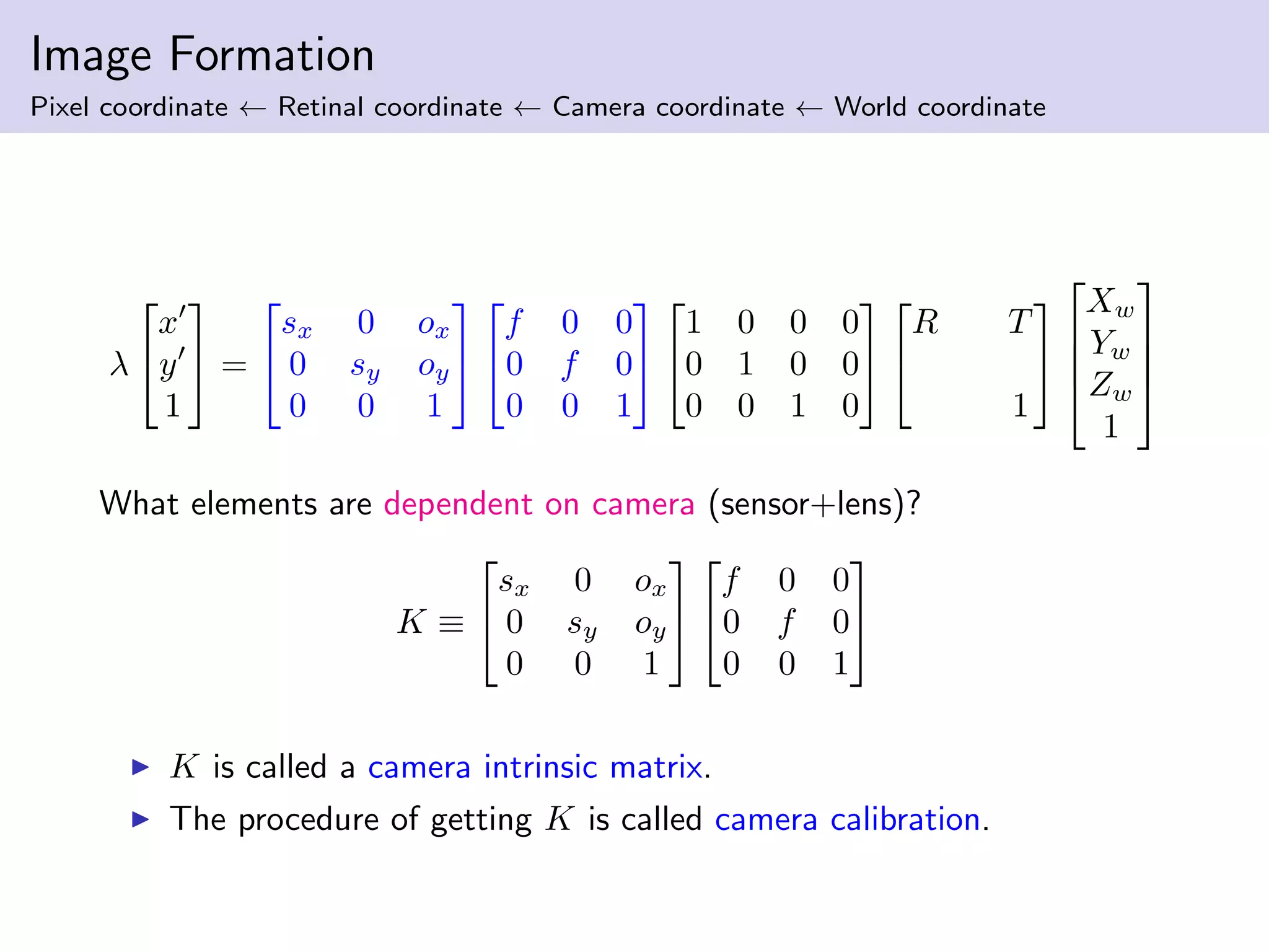
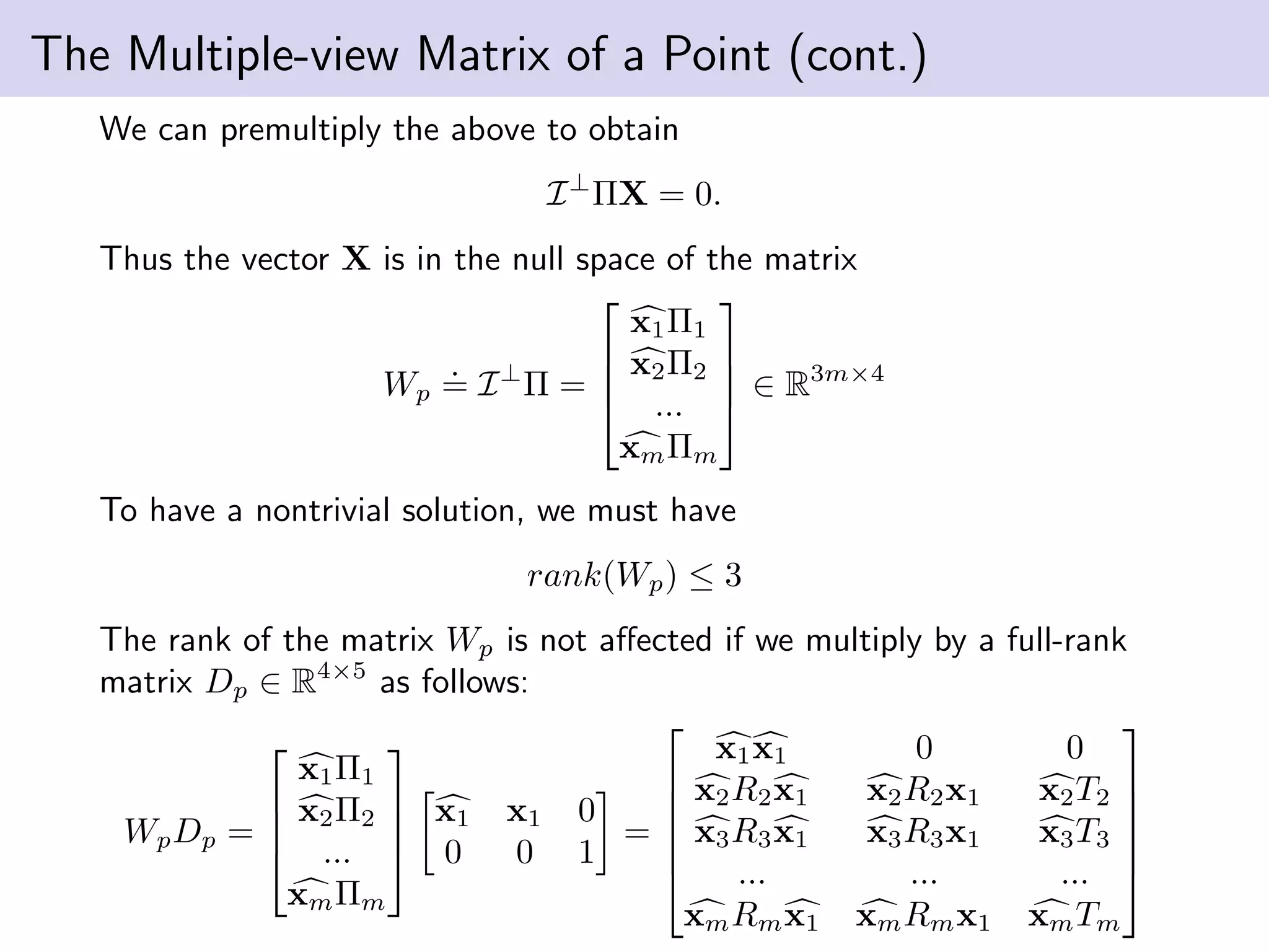
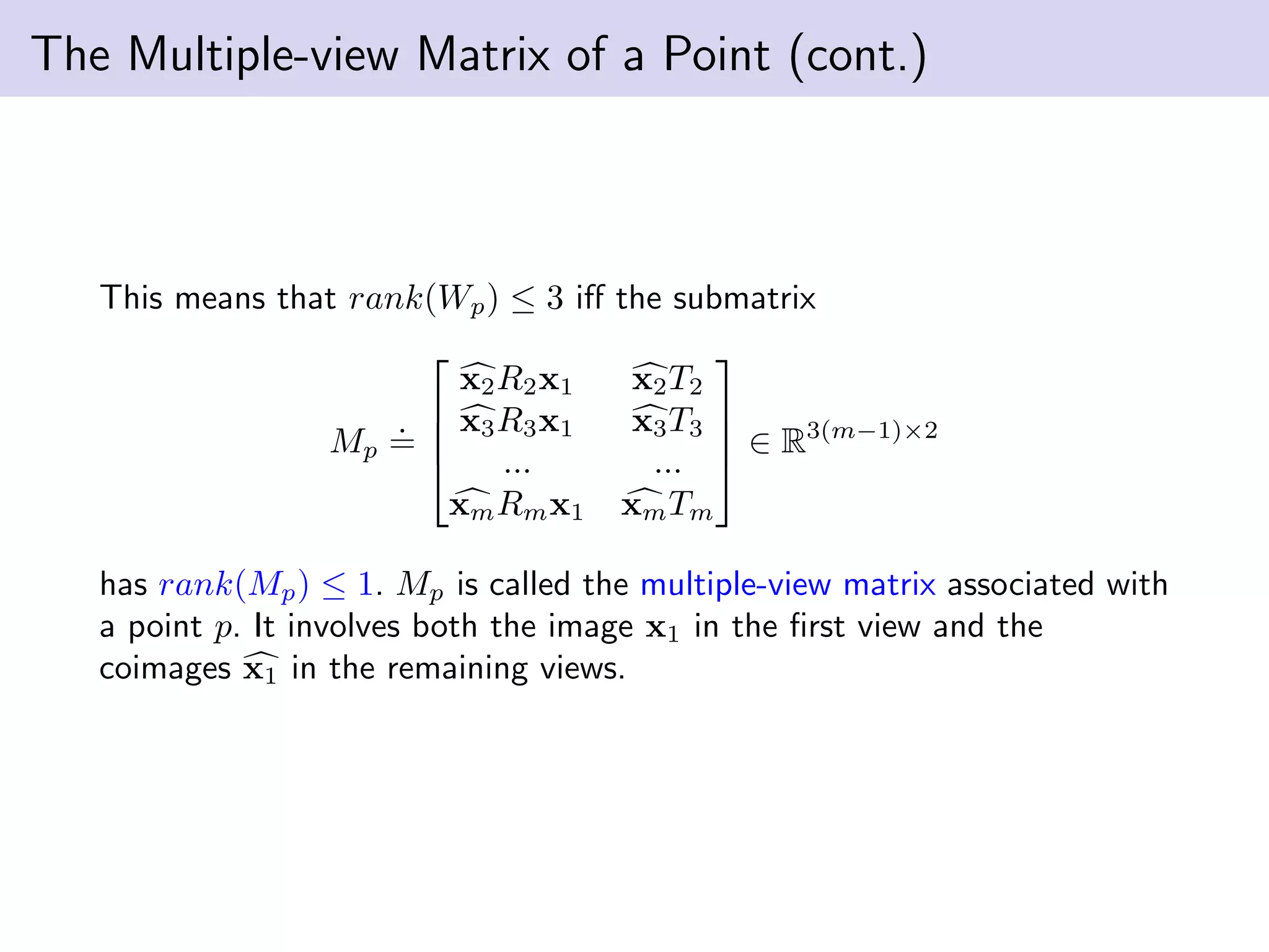
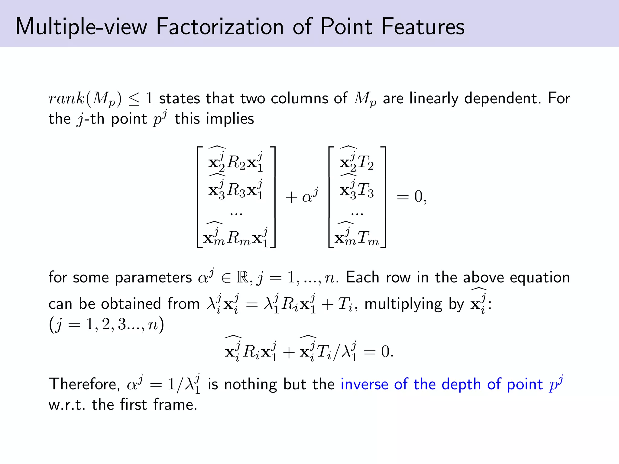
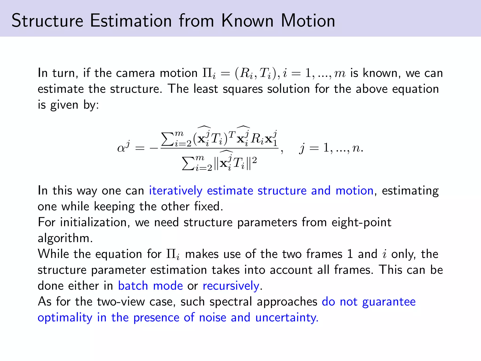
This document summarizes Ja-Keoung Koo's presentation on structure from motion. It discusses image formation, the structure from motion pipeline with calibrated cameras, and the 8-point algorithm. The key points are: 1. Image formation maps 3D world points to 2D image points using a camera's intrinsic and extrinsic parameters. 2. Structure from motion with calibrated cameras recovers 3D structure and camera motion from 2D correspondences using the essential matrix and 8-point algorithm. 3. The 8-point algorithm finds the essential matrix from point correspondences, decomposes it to recover the rotation and translation between views.


![Vibe Coding vs. Spec-Driven Development [Free Meetup]](https://cdn.slidesharecdn.com/ss_thumbnails/vibecodingvsspecdrivendevelopment-251209105622-43f455e7-thumbnail.jpg?width=640&height=640&fit=bounds)


