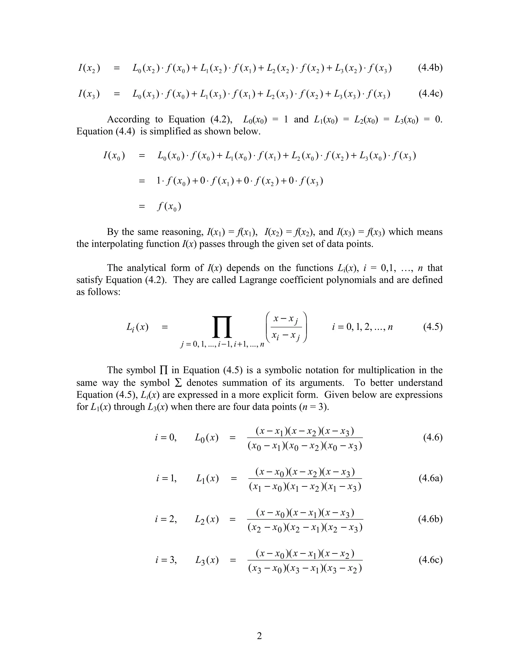
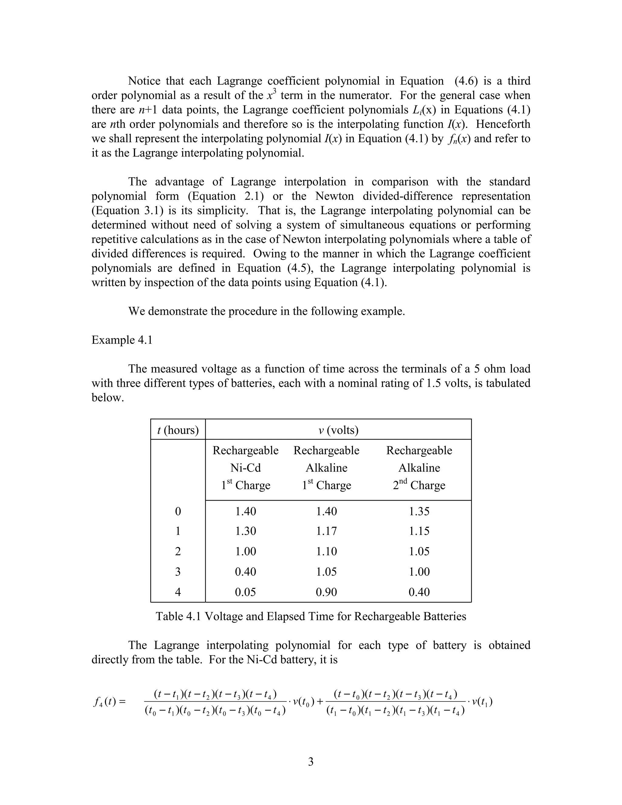
The document discusses Lagrange interpolating polynomials, which provide an alternative way to write an nth order polynomial that passes through a given set of n+1 data points. The Lagrange interpolating polynomial is defined as the sum of nth order Lagrange coefficient polynomials multiplied by the y-values at each data point. This allows the interpolating polynomial to be determined directly from the data points using simple formulas, without solving systems of equations. An example demonstrates computing the 4th order Lagrange interpolating polynomial for voltage data from three different batteries over time.

1. Section 4 Lagrange Interpolating Polynomials
In the previous sections we encountered two different ways of representing the
unique nth order (or lower) polynomial required to pass through a given set of n+1 points.
Yet another way of writing the polynomial, constrained in the same fashion, is presented
here. It is referred to as Lagrange's form of the interpolating polynomial.
Once again, we assume the existence of a set of data points (xi, yi), i = 0, 1, …, n
obtained from a function f(x) so that yi = f(xi), i = 0, 1, …, n. A suitable function for
interpolation I(x) is expressible as
n
I ( x) =
∑
i =0
Li ( x ) ⋅ f ( xi ) (4.1)
= L0 ( x ) ⋅ f ( x0 ) + L1 ( x ) ⋅ f ( x1 ) +.....+ Ln ( x ) ⋅ f ( x n ) (4.1a)
The functions Li(x), i = 0, 1, …, n are chosen to satisfy
R0
| x = x0 , x1 ,...., xi −1 , xi +1 ,...., xn U
|
L ( x) = S V (4.2)
i
|1
T x = xi |
W
Before we actually define the Li(x) functions, let's be certain we understand the
implications of Equations (4.1) and (4.2). The best way to accomplish this is simply to
choose a value for "n" and write out the resulting equations. Suppose we have the four
data points [xi, f(xi)], i = 0, 1, 2, 3. From Equations (4.1) with n = 3, the interpolating
function I(x) becomes
3
I ( x) =
∑
i=0
Li ( x ) ⋅ f ( xi ) (4.3)
= L0 ( x ) ⋅ f ( x 0 ) + L1 ( x ) ⋅ f ( x1 ) + L2 ( x ) ⋅ f ( x2 ) + L3 ( x ) ⋅ f ( x3 ) (4.3a)
and it remains to be shown that I(x) is identical to f(x) when x is any one of the four data
points. Evaluating I(x) at x0, x1, x2 and x3,
I ( x0 ) = L0 ( x0 ) ⋅ f ( x 0 ) + L1 ( x0 ) ⋅ f ( x1 ) + L2 ( x0 ) ⋅ f ( x 2 ) + L3 ( x 0 ) ⋅ f ( x3 ) (4.4)
I ( x1 ) = L0 ( x1 ) ⋅ f ( x0 ) + L1 ( x1 ) ⋅ f ( x1 ) + L2 ( x1 ) ⋅ f ( x2 ) + L3 ( x1 ) ⋅ f ( x3 ) (4.4a)
1

2. I ( x2 ) = L0 ( x 2 ) ⋅ f ( x 0 ) + L1 ( x 2 ) ⋅ f ( x1 ) + L2 ( x 2 ) ⋅ f ( x 2 ) + L3 ( x 2 ) ⋅ f ( x 3 ) (4.4b)
I ( x3 ) = L0 ( x 3 ) ⋅ f ( x 0 ) + L1 ( x 3 ) ⋅ f ( x1 ) + L2 ( x 3 ) ⋅ f ( x 2 ) + L3 ( x 3 ) ⋅ f ( x 3 ) (4.4c)
According to Equation (4.2), L0(x0) = 1 and L1(x0) = L2(x0) = L3(x0) = 0.
Equation (4.4) is simplified as shown below.
I ( x0 ) = L0 ( x 0 ) ⋅ f ( x 0 ) + L1 ( x 0 ) ⋅ f ( x1 ) + L2 ( x 0 ) ⋅ f ( x 2 ) + L3 ( x 0 ) ⋅ f ( x 3 )
= 1 ⋅ f ( x 0 ) + 0 ⋅ f ( x1 ) + 0 ⋅ f ( x 2 ) + 0 ⋅ f ( x 3 )
= f ( x0 )
By the same reasoning, I(x1) = f(x1), I(x2) = f(x2), and I(x3) = f(x3) which means
the interpolating function I(x) passes through the given set of data points.
The analytical form of I(x) depends on the functions Li(x), i = 0,1, …, n that
satisfy Equation (4.2). They are called Lagrange coefficient polynomials and are defined
as follows:
F x− xj I
Li ( x ) =
∏, i +1, ..., n GH xi − x j JK
j = 0, 1, ..., i − 1
i = 0, 1, 2, ..., n (4.5)
The symbol ∏ in Equation (4.5) is a symbolic notation for multiplication in the
same way the symbol ∑ denotes summation of its arguments. To better understand
Equation (4.5), Li(x) are expressed in a more explicit form. Given below are expressions
for L1(x) through L3(x) when there are four data points (n = 3).
( x − x1 )( x − x2 )( x − x3 )
i = 0, L0 ( x ) = (4.6)
( x0 − x1 )( x0 − x 2 )( x0 − x3 )
( x − x0 )( x − x2 )( x − x3 )
i = 1, L1 ( x ) = (4.6a)
( x1 − x 0 )( x1 − x2 )( x1 − x3 )
( x − x0 )( x − x1 )( x − x 3 )
i = 2, L2 ( x ) = (4.6b)
( x2 − x 0 )( x2 − x1 )( x2 − x3 )
( x − x0 )( x − x1 )( x − x2 )
i = 3, L3 ( x ) = (4.6c)
( x3 − x0 )( x3 − x1 )( x3 − x2 )
2

3. Notice that each Lagrange coefficient polynomial in Equation (4.6) is a third
order polynomial as a result of the x3 term in the numerator. For the general case when
there are n+1 data points, the Lagrange coefficient polynomials Li(x) in Equations (4.1)
are nth order polynomials and therefore so is the interpolating function I(x). Henceforth
we shall represent the interpolating polynomial I(x) in Equation (4.1) by fn(x) and refer to
it as the Lagrange interpolating polynomial.
The advantage of Lagrange interpolation in comparison with the standard
polynomial form (Equation 2.1) or the Newton divided-difference representation
(Equation 3.1) is its simplicity. That is, the Lagrange interpolating polynomial can be
determined without need of solving a system of simultaneous equations or performing
repetitive calculations as in the case of Newton interpolating polynomials where a table of
divided differences is required. Owing to the manner in which the Lagrange coefficient
polynomials are defined in Equation (4.5), the Lagrange interpolating polynomial is
written by inspection of the data points using Equation (4.1).
We demonstrate the procedure in the following example.
Example 4.1
The measured voltage as a function of time across the terminals of a 5 ohm load
with three different types of batteries, each with a nominal rating of 1.5 volts, is tabulated
below.
t (hours) v (volts)
Rechargeable Rechargeable Rechargeable
Ni-Cd Alkaline Alkaline
st
1 Charge 1st Charge 2nd Charge
0 1.40 1.40 1.35
1 1.30 1.17 1.15
2 1.00 1.10 1.05
3 0.40 1.05 1.00
4 0.05 0.90 0.40
Table 4.1 Voltage and Elapsed Time for Rechargeable Batteries
The Lagrange interpolating polynomial for each type of battery is obtained
directly from the table. For the Ni-Cd battery, it is
(t − t1 )(t − t 2 )( t − t 3 )( t − t 4 ) (t − t 0 )(t − t 2 )( t − t 3 )( t − t 4 )
f 4 (t ) = ⋅ v (t 0 ) + ⋅ v (t1 )
(t 0 − t1 )(t 0 − t 2 )( t 0 − t 3 )( t 0 − t 4 ) (t1 − t 0 )(t1 − t 2 )( t1 − t 3 )( t1 − t 4 )
3

4. (t − t 0 )(t − t1 )(t − t 3 )(t − t 4 ) (t − t 0 )(t − t 1 )(t − t 2 )(t − t 4 )
+ ⋅ v (t 2 ) + ⋅ v (t 3 )
(t 2 − t 0 )(t 2 − t1 )(t 2 − t 3 )(t 2 − t 4 ) (t 3 − t 0 )(t 3 − t 1 )(t 3 − t 2 )(t 3 − t 4 )
(t − t 0 )(t − t1 )(t − t 2 )(t − t 3 )
+ ⋅ v (t 4 ) (4.7)
(t 4 − t 0 )(t 4 − t1 )(t 4 − t 2 )(t 4 − t 3 )
(t − 1)(t − 2)(t − 3)(t − 4) t (t − 2)(t − 3)(t − 4)
f 4 (t ) = ⋅ 140 +
. ⋅ 130
.
(0 − 1)(0 − 2)(0 − 3)(0 − 4) (1 − 0)(1 − 2)(1 − 3)(1 − 4)
t (t − 1)(t − 3)(t − 4) t (t − 1)(t − 2)(t − 4)
+ ⋅ 100 +
. ⋅ 0.40
(2 − 0)(2 − 1)(2 − 3)(2 − 4) (3 − 0)(3 − 1)(3 − 2)(3 − 4)
t ( t − 1)( t − 2)( t − 3)
+ ⋅ 0.05 (4.8)
( 4 − 0)( 4 − 1)(4 − 2)( 4 − 3)
f 4 (t ) = 1.4 ( t − 1)(t − 2)(t − 3)(t − 4) − 163 t (t − 2)(t − 3)(t − 4) + 100 t (t − 1)(t − 3)(t − 4)
.
24 4
− 0.40 t ( t − 1)(t − 2)(t − 4) + 0.05 t ( t − 1)(t − 2)(t − 3) (4.9)
6 24
The same procedure is used to obtain the fourth order Lagrange interpolating
polynomials for the two alkaline batteries. Figure 4.1 shows the data points and the
fourth order interpolating polynomial for each battery.
It is generally advisable to begin with lower order polynomials for interpolation
and then increase the order in a systematic fashion until the results are acceptable. In
other words, a reduced subset of data points is chosen based on the expected range of the
interpolant. Suppose we have n+1 data points measured from a function f(x) where the
range of x is from xmin to xmax. Assuming interpolation over the entire interval is required
with a single polynomial, we might choose a third or possibly fourth order polynomial
(assuming n>4) based on a judicious choice of four or five points that include both
extremes. Visual inspection of the polynomial and its relationship to the entire set of data
points will determine if a higher order polynomial is required and which additional data
point should be included.
When an additional data point is required, the higher order polynomial will
generally exhibit more curvature than the previous one throughout the interpolation
interval. For example, Figure 4.2 shows polynomials of order n =1, 2, 3, and 4 required
to pass through data sets of two, three, four, and five points respectively
4

5. Alkaline,
1st Charge
Alkaline,
2nd Charge
Ni-Cd
Figure 4.1 Fourth Order Interpolating Polynomials For Battery Data in Table 4.1
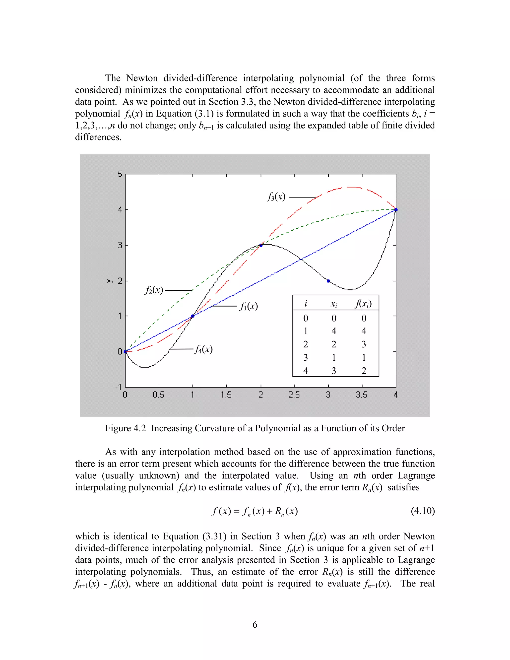
It's clear that the quadratic polynomial f2(x) exhibits more curvature than the
linear function f1(x) which of course has none. This is possible due to the presence of the
x2 term in f2(x). Similarly f3(x) curves more than f2(x) due to the additional point [x3,
f(x3)] and the fourth order term x4 in f4(x) accounts for the added curvature compared to
f3(x) over the interval (0,4).
With an nth interpolating polynomial in standard form, Equation (2.1), or the
Newton divided-difference form, Equation (3.1), there is only one high order term, i.e. a
single term with xn. This is in contrast to the Lagrange form of the interpolating
polynomial, Equation (4.1), in which each term of the overall expression is an nth order
polynomial. If the order of the interpolating polynomial is to be increased from n to n+1
by including an additional data point, each Lagrange coefficient polynomial in Equation
(4.5) increases in order from n to n+1 as well. Consequently, the entire Lagrange
interpolating polynomial must be recomputed.
Despite the fact interpolating polynomials in standard form contain a single high
order term, an extra data point requires recalculation of all the coefficients ai, i = 0,1,2,
…, n in addition to the new coefficient an+1. The system of equations to be solved was
considered in Section 3.2 and enumerated in matrix form in Equation (2.3). The
Vandermonde matrix and the column vectors of coefficients and function values in
Equation (2.3) are (n+1) × (n+1), n × 1, and n × 1, respectively.
5

6. The Newton divided-difference interpolating polynomial (of the three forms
considered) minimizes the computational effort necessary to accommodate an additional
data point. As we pointed out in Section 3.3, the Newton divided-difference interpolating
polynomial fn(x) in Equation (3.1) is formulated in such a way that the coefficients bi, i =
1,2,3,…,n do not change; only bn+1 is calculated using the expanded table of finite divided
differences.
f3(x)
f2(x)
f1(x) i xi f(xi)
0 0 0
1 4 4
f4(x) 2 2 3
3 1 1
4 3 2
Figure 4.2 Increasing Curvature of a Polynomial as a Function of its Order
As with any interpolation method based on the use of approximation functions,
there is an error term present which accounts for the difference between the true function
value (usually unknown) and the interpolated value. Using an nth order Lagrange
interpolating polynomial fn(x) to estimate values of f(x), the error term Rn(x) satisfies
f ( x ) = f n ( x ) + Rn ( x ) (4.10)
which is identical to Equation (3.31) in Section 3 when fn(x) was an nth order Newton
divided-difference interpolating polynomial. Since fn(x) is unique for a given set of n+1
data points, much of the error analysis presented in Section 3 is applicable to Lagrange
interpolating polynomials. Thus, an estimate of the error Rn(x) is still the difference
fn+1(x) - fn(x), where an additional data point is required to evaluate fn+1(x). The real
6

7. advantage of Newton divided-difference interpolating polynomials is the reduced
computational effort (compared with the Lagrange form) to obtain fn+1(x) when fn(x) is
already computed.
Example 4.2
In Example 4.1, estimate the error incurred by the use of a fourth order Lagrange
interpolating polynomial for approximating the voltage of a Ni-Cd battery after 1.5
hours. Assume an additional data point is available, namely t = 2.5 hours, v = 0.7 volts.
From Equation (4.9),
f 4 (15) =
. 1.4 (15 − 1)(15 − 2)(15 − 3)(15 − 4) − 1.3 15(15 − 2)(15 − 3)(15 − 4)
24 . . . . 6 . . . .
+ 100 15(15 − 1)(15 − 3)(15 − 4) − 0.6 15(15 − 1)(15 − 2)(15 − 4)
40 . .
4 . . . . . .
+ 0.05 15(15 − 1)(15 − 2)(15 − 3)
24 . . . .
f 4 (15) =
. 11965
.
Supplementing Table 4.1 with the new data point and determining the fifth order
Lagrange interpolating polynomial yields,
(t − 1)(t − 2)(t − 3)(t − 4)(t − 2.5) t (t − 2)(t − 3)(t − 4)(t − 2.5)
f 5 (t ) = ⋅ 140 +
. ⋅ 130
. (4.11)
(0 − 1)(0 − 2)(0 − 3)(0 − 4)(0 − 2.5) (1 − 0)(1 − 2)(1 − 3)(1 − 4)(1 − 2.5)
t (t − 1)(t − 3)(t − 4)(t − 2.5) t (t − 1)(t − 2)(t − 4)(t − 2.5)
+ ⋅ 100 +
. ⋅ 0.40
(2 − 0)(2 − 1)(2 − 3)(2 − 4)(2 − 2.5) (3 − 0)(3 − 1)(3 − 2)(3 − 4)(3 − 2.5)
t (t − 1)( t − 2)( t − 3)( t − 2.5) t ( t − 1)( t − 2)(t − 3)( t − 4)
+ ⋅ 0.05 + 0.70
( 4 − 0)( 4 − 1)( 4 − 2)( 4 − 3)( 4 − 2.5) ( 2.5 − 0)(2.5 − 1)(2.5 − 2)( 2.5 − 3)( 2.5 − 4)
R4(1.5) is the difference between the true (unknown) function value f(1.5) and the
fourth order interpolating polynomial estimate f4(1.5), i.e.
R4 (15) =
. f (15) − f 4 (15)
. .
We can estimate R4(1.5) using
R4 (15) ≈
. f 5 (15) − f 4 (15)
. .
≈ 12148 − 11965
. .
≈ 0.0184
7

8. Exercises
1. A simplified mathematical model of traffic flow is based on the assumption that at
any point along a road, the velocity of a car depends only on the density of cars in the
immediate vicinity. At low densities, drivers are free to drive at their desired speed,
called the mean free speed. At high densities, vehicle speeds are lower, ultimately
approaching zero at the maximum density corresponding to bumper-to-bumper traffic.
This model is applicable on single lane roads or tunnels where car passing is not
allowed.
Measurements of average velocity (in mph) and traffic density (vehicles/mile) were
taken in a tunnel to determine its velocity-density profile.
Density, ρ Velocity, u
(vehicles/mile) (mph)
20.5 39.8
31.2 30.9
50.4 22.7
86.4 13.1
120.9 6.2
160.0 4.3
Data for Problem 1
a) Graph the data points.
b) Find a third order Lagrange polynomial u = f3(ρ) suitable for interpolation over
the entire range of densities. Plot the polynomial on the same graph as the data
points.
c) Calculate the true error f(ρ) - f3(ρ), where u = f(ρ) is the true function, at the two
remaining data points.
d) Estimate the average speed of traffic when the mile and a half long tunnel has 75
cars uniformly spaced in it.
e) Suppose the speed limit in the tunnel is 35 mph. Estimate the uniform traffic
density throughout the tunnel at which traffic tends to flow at the speed limit.
f) The traffic flow q (vehicles/hr) through the tunnel under steady-state conditions
(uniform density and constant speed) is the product of traffic density, ρ
(vehicles/mile) and vehicle speed, u (miles/hr). Generate a graph of q vs. ρ for the
tunnel using the Lagrange polynomial from Part b). Traffic engineers refer to this
as the Fundamental Diagram of Traffic Flow.
8

9. g) The maximum traffic flow is called the capacity of the road. Estimate the tunnel's
capacity. What should the posted speed limit be to achieve this capacity?
2. The field strength of the earth's gravitational field g diminishes with distance h from
the surface of the earth. The following table shows the field strength at several
distances.
Distance, h Field Strength, g Distance, h Field Strength, g
(106 m) (N/kg) (106 m) (N/kg)
0 9.81 20 0.58
2.5 5.07 30 0.30
5 3.09 40 0.19
10 1.49 50 0.12
Data for Problem 2
a) Plot the data points.
b) An interpolating polynomial is required to estimate g from zero to 20 ×106 m.
Find the Lagrange interpolating polynomial f7(h) which passes through all the
data points and the Lagrange interpolating polynomial f4(h) which passes through
the first five data points. Plot both over the interval 0 ≤ h ≤ 20×106 m and
comment on which is more suitable for interpolation.
c) Estimate the distance from earth where a 1 kg mass weighs 2 Newtons, i.e. where
the gravitational field strength is 2 N/kg, using the two interpolating polynomials
form Part b).
d) The true function relating g and h is
GmE
g = f ( h) =
b R + hg
E
2
where G = 6.7×10-11 N⋅m2/kg2 (gravitational constant)
mE = 6.0×1024 kg (mass of the earth)
RE = 6.4×106 m (radius of the earth)
Plot the true function f(h) on the same graph as the data points and the
interpolating polynomials f4(h) and f7(h) over the interval 0 ≤ h ≤ 50×106 m.
Comment on the suitability of either interpolating polynomial over the entire
interval 0 ≤ h ≤ 50×106 m.
e) Calculate the true errors in the two estimates of g in Part c).
9

10. f) Try to find an interpolating polynomial that can be used to provide reasonably
accurate estimates of g over the entire interval 0 ≤ h ≤ 50×106 m. Generate more
data points from the true function g = f(h) if you think this will help.
g) Use an appropriate Lagrange interpolating polynomial to estimate the distance
from the earth's surface where you weigh one half of your weight on earth.
h) Calculate the error in the estimated distance in Part g).
3. The curves shown below are the trajectories of a batted baseball thrown at 85 mph
with a bat speed of 70 mph directed upward by 10 degrees. The various curves
correspond to the amount that the bat is swung under the ball. For example, the case
when the underswing is ¾ inches is illustrated in the upper corner.
(Source: Falk Sport Facts, F.W. Roth, 1991)
Graphs for Problem 3
a) Select one of the curves and generate a set of tightly spaced data points sampled
from the curve. Represent the actual curve by a piecewise linear approximation
through the data points. Graph the approximating function, which should appear
smooth, as a dotted curve without showing the data points. Label it H = f(D).
b) For the same curve selected in Part a) generate a reduced set of sampled data
points (no more than 10) that captures the basic profile of the curve.
c) Try to fit a Lagrange interpolating polynomial fn(D) over the entire interval
represented by the data points. Plot the piecewise function f(D), the interpolating
polynomial fn(D) and the data points on the same graph.
10

11. 4. An electronics lab experiment was designed to compare the measured voltage-current
relationship for a light emitting diode with calculated values based on the known
nonlinear resistance characteristic of the diode. Results are given in the table below.
(Source: Monaghan, Computers in Education, Jan-Mar 1998)
VOLTAGE VS. CURRENT FOR A LIGHT EMITTING DIODE
LAB MEASUREMENTS CALCULATED VALUES
VOLTAGE CURRENT VOLTAGE CURRENT
(volts) (milliamperes) (volts) (milliamperes)
1.421 0.095 1.420 0.118
1.441 0.155 1.440 0.186
1.446 0.281 1.460 0.295
1.487 0.461 1.480 0.468
1.512 0.808 1.500 0.741
1.535 1.390 1.520 1.173
1.556 2.350 1.540 1.859
1.557 4.080 1.560 2.944
1.596 6.720 1.580 4.664
Table for Problem 4
a) Plot the measured and calculated current vs. voltage data points on separate
graphs.
b) Find second, third and fourth order Lagrange interpolating polynomials for each
set based on the following data points.
MEASURED:
ORDER DATA POINTS
2 (1.421,0.095),(1.512, 0.808),(1.596,6.720)
3 (1.421,0.095),(1.487, 0.461),(1.535,1.390),(1.596,6.720)
4 (1.421,0.095),(1.446, 0.281),(1.512, 0.808), 1.556, 2.350),(1.596,6.720)
CALCULATED:
ORDER DATA POINTS
2 (1.420,0.118), (1.500, 0.741), (1.580,4.664)
11

12. 3 (1.420,0.118), (1.480, 0.468), (1.520,1.173), (1.580,4.664)
4 (1.420,0.118),(1.460, 0.295),(1.500, 0.741),(1.540,1.859), (1.580,4.664)
c) Plot the polynomials on the same graphs with the data points. Comment on the
results.
d) Denote i = f(vi) as the function relating the actual measured current and voltage.
Calculate the average error for each interpolating polynomial fn(vi) i.e.
9
Eave = 1
9 ∑ f (vi ) − f n (vi ) , n = 2,3,4
i =1
e) Repeat Part d) with i = f(vi) as the function relating the actual calculated current
and voltage.
5. The displacement diagram for a disk cam with reciprocating follower is shown in the
figure.
Lift x vs. Cam Angle θ
x = f(θ)
180 ≤ θ ≤ 220
θ
Figure for Problem 5
a) Generate two sets of data points (θi, xi) one for cam angles θi between 0 and 180
degrees, the other for cam angles between 220 and 360 degrees. Choose the
points so that Lagrange interpolating polynomials can be used to approximate
both profiles. Plot both sets of data points on the same graph.
12

13. b) Find the lowest order Lagrange interpolating polynomials that describe both
profiles reasonably well. (They do not have to be the same order)
c) Plot the polynomials from Part b) on the same graph as the data points.
d) Select several additional data points from both profiles and calculate the true error
f(θi)- fn(θi), where n is the order of the polynomial, at each of those points.
6. A car buyer is financing the purchase of a $35,000 automobile. The bank has several
loan packages to choose from. The choices are summarized below.
Loan Period Annualized Interest rate Monthly Payment
n (months) i (%) A ($)
24 5.0 1535.50
36 5.5 1056.86
48 6.0 821.86
60 6.5 684.82
72 7.0 596.72
Table for Problem 6
a) Plot the data points (nk, Ak), k = 1,2,3,4,5.
b) Find the 4th order Lagrange interpolating polynomial A = f4(n) through the data
points and plot it on the same graph.
c) The bank is willing to write the loan for any number of months between 24 and
72. Estimate the monthly payment if the car buyer chooses a three and a half year
loan.
d) The interest rate on the loan increases with the duration of the loan. Use the table
to interpolate i(42), the annualized per cent interest rate for a forty-two month
loan.
e) The formula for calculating the monthly payment A given the amount financed P,
the annual per cent interest rate i, and the loan duration n in months, is
A = f ( P , i , n) = P
LM (1 + ) OP
i
1200
i
1200
n
N (1 + ) − 1 Q
i
1200
n
Find the true error in the estimated monthly payment f4(42) calculated in Part c),
i.e. f(35000, i(42), 42) - f4(42).
f) The car buyer can afford monthly payments of $770. Use the graph A = f4(n) to
estimate (to the nearest month) the loan duration requiring this amount of
payment.
13

14. g) Find the true loan duration (to the nearest month) when the monthly payment is
$770. and compare the result to the answer in Part f). Hint: You will need to
solve A = f(P, i, n) for n by trial and error since i is unknown as well.
7. The estimated net lifetime benefits (in inflation adjusted 1993 dollars) for social
security recipients born in different years is tabulated below.
(Source: U.S. News and World Report, April 20, 1998)
Birth Year Net Lifetime Benefits
1885 $29,000
1900 $51,000
1915 $60,000
1930 $14,000
1945 -$18,000
1960 -$33,000
1975 -$32,000
1985 -$31,000
Data for Problem 7
a) Graph the data points.
b) Find the seventh order Lagrange interpolating polynomial passing through the
data points and plot it on the same graph.
c) Estimate the year of birth for a social security recipient to have net benefits of
zero.
d) Estimate the maximum net lifetime social security benefits and the year of birth
for recipients receiving the maximum.
8. Consider the 3 points from the function f(x) = ex in the table below.
i xi yi = f(xi)
0 ln1 1
1 ln12 12
2 ln7 7
Table for Problem 8
a) Find the first order Lagrange polynomial f1(x) to be used for estimating f(ln5).
14

15. b) Find the second order Lagrange polynomial f2(x) to be used for estimating f(ln5).
c) Plot the given data points and both interpolating polynomials on the same graph.
d) Calculate the interpolation errors Ri(ln5) = f(ln5) - fi(x), i = 1, 2.
9. Railroad freight traffic measured in billions of ton-miles since 1965 is presented in
tabular form. (Source: Assoc. of American Railroads)
Year 1965 1970 1975 1980 1985 1990 1995
Traffic 700 750 750 925 850 980 1275
Data Points for Problem 9
Estimate the year between 1975 and 1985 when the freight traffic was a maximum
and the amount of traffic in that year.
10. The following data points were obtained from a function y = f(x).
x 0 1 2 3 4 5 6 7 8 9 10
f(x) -10 -8 -6 -4 -2 0 2 4 6 8 10
a) Plot the points.
b) Find the lowest order Lagrange interpolating polynomial through the entire set of
data points and plot it on the same graph.
c) Suppose the middle data point was incorrectly obtained as (5, y) where y = 0.5.
Find the lowest order interpolating polynomial fn(x), n ≤ 10, through the entire set
of data points and plot it on the same graph. The interpolating polynomial may be
expressed in standard form.
d) Find the second order Lagrange interpolating polynomial f2(x) through the end
points and the new middle data point and plot it on the same graph.
e) Assuming the function f(x) is linear, calculate the true error at x = 0.4 and x =
4.75 resulting from the use of both polynomials.
f) Repeat Parts c), d) and e) for y = -1 and 2.
g) Comment on the results.
15