This document discusses the relationship between cellular automata (CA), partial differential equations (PDEs), and pattern formation. It begins by introducing CA as a rule-based computing system and noting that CA and PDE models both describe temporal evolution, raising the question of how to relate the two approaches. The document then covers the fundamentals of CA, including finite-state CA, stochastic CA, and reversible CA. It discusses using CA to model PDEs by constructing CA rules from finite difference schemes. Finally, it discusses how both CA and PDEs can be used to model pattern formation in various natural and engineered systems.

1. 18
Cellular Automata,
PDEs, and
Pattern Formation
Xin-She Yang and
Y. Young
18.1 Introduction. . . . . . . . . . . . . . . . . . . . . . . . . . . . . . . . . . . . . . . . . . . . . . 18-271
18.2 Cellular Automata . . . . . . . . . . . . . . . . . . . . . . . . . . . . . . . . . . . . . . . 18-272
Fundamentals of Cellular Automaton • Finite-State Cellular
Automata • Stochastic Cellular Automata • Reversible
Cellular Automata
18.3 Cellular Automata for Partial Differential
Equations . . . . . . . . . . . . . . . . . . . . . . . . . . . . . . . . . . . . . . . . . . . . . . . . . 18-274
Rules-Based System and Equation-Based System • Finite
Difference Scheme and Cellular Automata • Cellular
Automata for Reaction-Diffusion Systems • CA for the
Wave Equation • Cellular Automata for Burgers Equation
with Noise
18.4 Differential Equations for Cellular Automata. . . . . . . . . . 18-277
Formulation of Differential Equations from Cellular
Automata • Stochastic Reaction-Diffusion
18.5 Pattern Formation . . . . . . . . . . . . . . . . . . . . . . . . . . . . . . . . . . . . . . . 18-278
Complexity and Pattern in Cellular Automata • Comparison
of CA and PDEs • Pattern Formation in Biology and
Engineering
References . . . . . . . . . . . . . . . . . . . . . . . . . . . . . . . . . . . . . . . . . . . . . . . . . . . . . . . 18-281
18.1 Introduction
A cellular automaton (CA) is a rule-based computingmachine,whichwas first proposed by vonNewmann
in early 1950s and systematic studies were pioneered by Wolfram in 1980s. Since a cellular automaton
consists of space and time, it is essentially equivalent to a dynamical system that is discrete in both space
and time. The evolution of such a discrete system is governed by certain updating rules rather than
differential equations. Although the updating rules can take many different forms,most common cellular
automata use relatively simple rules. On the other hand, an equation-based system such as the system
of differential equations and partial differential equations also describe the temporal evolution in the
domain. Usually, differential equations can also take different forms that describe various systems. Now
one natural question iswhat is the relationship between a rule-based systemand an equation-based system?
CHAPMAN: “C4754_C018” — 2005/5/5 — 22:53 — page 271 — #1
18-271

2. 18-272 Handbook of Bioinspired Algorithms and Applications
f1(t ) fi –2(t ) fi –1(t )
fi (t ) fi +1 (t) fi –2 (t ) fN (t ) • • • • • •
fi (t +1)
FIGURE 18.1 Diagram of a one-dimensional cellular automaton.
Given differential equations, how can one construct a rule-based cellular automaton, or vice versa? There
has been substantial amount of research in these areas in the past two decades. This chapter intends
to summarize the results of the relationship among the cellular automata, partial differential equations
(PDEs), and pattern formations.
18.2 Cellular Automata
18.2.1 Fundamentals of Cellular Automaton
On a one-dimensional (1D) grid that consists of N consecutive cells, each cell i (i = 1, 2, . . . ,N) may be
at any of the finite number of states, k. At each time step, t , the next state of a cell is determined by its
present state and the states of its local neighbors. Generally speaking, the state φi at t + 1 is a function of
its 2r + 1 neighbors with r cells on the left of the concerned cell and r cells on its right (see Figure 18.1).
The parameter r is often referred to as the radius of the neighborhood.
The number of possible permutations for k finite states with a radius of r is p = k2r+1, thus the
number of all possible rules to generate the state of cells at next time step is kp, which is usually very large.
For example, if r = 2, k = 5, then p = 125 and the number of possible rules is 5125 ≈ 2.35×1087, which
is much larger than the number of stars in the whole universe.
The rule determining the new state is often referred to as the transition rule or updating rule.
In principle, the state of a cell at next time step can be any function of the states of some neighbor
cells, and the function can be linear and nonlinear. There is a subclass of the possible rules according
to which the new state depends only on the sum of the states in a neighborhood, and this will simplify
the rules significantly. For this type of updating rules, the number of possible permutations for k states
and 2r + 1 neighbors is simply k(2r + 1), and thus the number of all possible rules is kk(2r+1). Then
for the same parameter k = 5, r = 2, the number of possible rules is 515 = 3.05 × 1010, which is much
smaller when compared with 5125. This subclass of sum-rule or totalistic rule is especially important in the
popular cellular automata such as Conway’s Game of Life, and in the cellular automaton implementation
of partial differential equations.
The dynamics and complexity of cellular automata are extremely rich. Stephan Wolfram’s pioneering
research and mathematical analysis of cellular automata led to his famous classification of 1D cellular
automata:
Class 1: The first class of cellular automata always evolves after a finite number of steps from almost
all initial states to a homogeneous state where every cell is in the same state. This is something like
fixed point equilibrium in the dynamical system.
Class 2: Periodic structures with a fixed number of states occur in the second class of cellular automata.
Class 3: Aperiodic or “chaotic” structures appear from almost all possible initial states in this type of
cellular automata.
Class 4: Complex patterns with localized spatial structure propagate in the space as time evolves.
Eventually, these patterns will evolve to either homogeneous or periodic. It is suggested that this
class of cellular automata may be capable of universal computation.
Cellular automata can be formulated in higher dimensions such as 2D and 3D. One of the most
popular and yet very interesting 2D cellular automata using relatively simple updating rules is the
CHAPMAN: “C4754_C018” — 2005/5/5 — 22:53 — page 272 — #2

3. Cellular Automata, PDEs, and Pattern Formation 18-273
Conway’s Game of Life. Each cell has only two states k = 2, and the states can be 0 and 1. With a
radius of r = 1 in the 2D case, each cell has eight neighbors, thus the new state of each cell depends on
total nine cells surrounding it. The boundary cells are treated as periodic. The updating rules are: if two
or three neighbors of a cell are alive (or 1) and it is currently alive, then it is alive at next time step; if three
ij7→ φt+1
CHAPMAN: “C4754_C018” — 2005/5/5 — 22:53 — page 273 — #3
AQ: Please
Check if change
is ok in the
sentence ‘The
updating rules
are: if two or...’.
neighbors of a cell are alive (or 0) and it is currently not alive its next state is alive; the next state is not
alive for all the other cases. It is suggested that this simple automaton may have the capability of universal
computation. There are many existing computer programs such as Life inMatlab and screen savers on all
computer platforms such asWindows and Unix.
18.2.2 Finite-State Cellular Automata
In general, we can define a finite-state cellular automaton with a transition rule G = [gij,...,l ], (i, j, . . . , l =
1, 2, . . . ,N) from one state 8t = [φt
ij,...,l ] at time level n to a new state 8t+1 = [φt+1
ij,...,l ] at a new time step
n + 1. The value of subscript (i, j, . . . , l) denotes the dimension, d, of the cellular automaton. Therefore,
a CA in the d-dimensional space has Nd cells. For the 2D case, this can be written as
G : 8t7→ 8t+1, gij : φt
ij , (i, j = 1, 2, . . . ,N).
In the case of sum-rule with a 4r + 1 neighbors, this becomes
φt+1
ij = G
µ Xr
α=−r
Xr
β=−r
aαβ φt
i+α, j+β
¶
, (i, j = 1, 2, . . . ,N),
where aαβ (α, β = ±1,±2, . . . ,±r) are the coefficients. The cellular automata with fixed rules defined
this way are deterministic cellular automata. In contrast, there exists another type, namely, the stochastic
cellular automata that arise naturally from the stochastic models for natural systems (Guinot, 2002;
Yang, 2003).
18.2.3 Stochastic Cellular Automata
When using cellular automata to simulate the phenomena with stochastic components or noise such as
percolation and stochastic process, themore effective way is to introduce some probability associated with
certain rules. Usually, there is a set of rules and each rule is applied with a probability (Guinot, 2002).
Another way is that the state of a cell is updated according to a rule only if certain conditions are met or
AQ: Please check
the change in
the sentence
‘Another way
is...’.
certain values are reached for some random variables. For example, the rule for 2D a cellular automaton
g (φt
ij ) = φt+1
ij is applied at a cell only if a random variable v ≤ Ŵ(φt
ij ) where the function Ŵ ∈ [0, 1].
At each time step, a randomnumber v is generated for each cell (i, j), and the new statewill be updated only
if the generated random number is greater than Ŵ, otherwise, it remains unchanged. Cellular automata
constructed this way are called stochastic or probabilistic cellular automata. An example is given later in
the next section.
18.2.4 Reversible Cellular Automata
A cellular automaton with an updating rule φt+ ij = g (φt
ij ) is generally irreversible in the sense that it is
impossible to know the states of a region such as all zeros were the same at a previous time step or not.
However, certain class of rules will enable the automata to be reversible. For example, a simple finite
AQ: Should
‘φt+ ij ’ be ‘φt+1
ij ’
in the sentence
‘A cellular
automata...’.
Please check.
difference (FD) scheme for a dynamical system
u(t + 1) = g [u(t )] − u(t − 1) or u(t − 1) = g [u(t )] − u(t + 1),

4. 18-274 Handbook of Bioinspired Algorithms and Applications
is reversible since for any function g (u), one can compute u(t + 1) from u(t ) and u(t − 1), and invert
u(t − 1) from u(t ) and u(t + 1). The automaton rule for 2D reversible automata can be similarly
constructed as
ut+1
i,j = g (ut
i,j ) − ut−1
i,j ,
together with appropriate boundary conditions such as fixed-state boundary conditions (Margolus, 1984).
18.3 Cellular Automata for PDEs
Cellular automata have been used to study many phenomena (Vichniac, 1984; Wolfram, 1984, 1994;
Weimar, 1997; Yang, 2002). In fact, many natural phenomena behave like finite-state AQ: Please specify if cellular automata,
Wolfram 1984 is
1984a or 1984b.
and these include self-organized systems such as pattern formation in biological system, insect colonies,
and ecosystem;multiple particle systemsuch as the lattice-gas, granularmaterial, and fluids; autocatalytic
systems such as enzyme functionality and mineral reactions; and even systems involving society and
culture interactions.However,most of these systems have been studied using continuum-based differential
equations.We now focus on the formulation of automaton rules from corresponding PDEs.
18.3.1 Rules-Based System and Equation-Based System
Equation-based relationships, often in the form of ordinary differential equations and partial differential
equations, form the continuum models of most physical, chemical, and biological processes. Differential
equations are suitable and work well for systems with only a small degree of freedom and evolution of
system variables in the continuous and smooth manner. There have been vast literatures on analysis and
solution technique of the differential models. On the other hand, cellular automata are often considered
as an alternative approach and may compliment the existing mathematical basis. The state variables are
AQ: Please specify if
Wolfram 1984 is
1984a or 1984b. always discrete, but the numbers of degree of freedom are large (Wolfram, 1984).
Although continuum models have advantages such as high accuracy and conservation laws, mathe-matical
analysis are usually very difficult and the analytical solutions do not always exist. Only few
differential equations have a closed-form solution. In last several decades, the numerical methods have
become the essential parts of the solution and of the analysis of almost all problems in engineering,
physics, and biology. In fact, computational modeling and numerical computation have become the third
component, bridging the gap between theoretical models and experiments. As the computing speed and
memory of computers increase, computer simulations have become a daily routine in science and engi-neering,
especially in multidisciplinary research. There are also vast literatures concerning the numerical
algorithms, numerical solutions of partial differential equations, and others. These include the following
well-established methods: finite differencemethod, finite elementmethod, finite volumemethod, cellular
automata, lattice-gas,Monte-Carlo method, and genetic algorithms.
Finite difference methods work very well for many problems, but have disadvantages in dealing with
irregular geometry. Finite element and finite volume methods can deal with irregular geometry and thus
are commonly used and there are quite a few commercial software packages available. Lattice-gas and
Monte-Carlo methods are suitable for many problems in physics, especially for systems with multibodies
or multiparticles. Cellular automaton is a very interesting and powerful method, and it has gradually
become an essential part of the numerical computations owing to its universal computability and the
nature of parallel implementation.
18.3.2 Finite Difference Scheme and Cellular Automata
There is a similarity between finite difference scheme and finite-state cellular automata. Finite difference
scheme is the discretization of a differential equation on a regular grid of points with the evolution of the
states over the discrete time steps. Even the state variable froma differential equation may have continuous
CHAPMAN: “C4754_C018” — 2005/5/5 — 22:53 — page 274 — #4

5. Cellular Automata, PDEs, and Pattern Formation 18-275
values; numerical computation on a computer always lead to the discrete values due to the limited bits of
processors or round-off. Similarly, cellular automata are also about the evolution of state variables with
finite number of values on a regular grid of cells at different discrete time steps. If the number of states of
a cellular automaton is comparable with that of the related finite difference equation, then we can expect
the results to be comparable.
To demonstrate this, we choose the 1D heat equation
∂T
∂t = κ
∂2T
∂x2 ,
where T is temperature and κ is the thermal diffusivity. This is a mathematical model that is widely used
to simulate many phenomena. The temperature T(x, t ) is a real-valued function, and it is continuous
for any time t > 0 whatever the initial conditions. In reality, it is impossible to measure the temperature
at a mathematical point, and the temperature is always the average temperature in a finite representative
volume over certain short time.Mathematically, one can obtain a closed-formsolution with infinite accu-racy
in the domain, but physically the temperature would only be meaningful at certain macroscopic
levels. No matter how accurate the solution may have at very fine scale, it would be meaningless to try
to use the solution at the atomic or subatomic levels where quantum mechanics come into play and, the
CHAPMAN: “C4754_C018” — 2005/5/5 — 22:53 — page 275 — #5
AQ: Toffili, 1984
has been change
to Toffoli as per
the Ref. list.
Trust it is ok.
solution of temperature is invalid (Toffoli, 1984). Thus, numerical computation would be very useful even
though it has finite discrete values.
The simplest discretization of the above heat equation is the central difference for spatial derivative and
forward scheme for time derivatives, and we have
Tn+1
i − Tn
i =
κ1t
(1x)2
(Tn
i+1 − 2Tn
i + Tn
i−1),
where i and n are the spatial and time indices. If we choose the time steps and spatial discretization such
that κ1t/(1x)2 = 1, now we have
Tt+1
i = (Tt
i+1 + Tt
i + Tt
i−1) − 2Tt
i ,
which is something like the “mod 2” cellular automata or Wolfram’s cellular automata with rule 150
AQ: Please
specifyWolfram
1984a or b.
(Wolfram, 1984;Weimar, 1997).
Cellular automata obtained thisway are very similar to the finite differencemethod. If the state variables
are discrete, they are exactly the finite-state cellular automata. However, one can use the continuous-valued
state variable for such simulation, in this case, they are continuous-valued cellular automata from
differential equations as studied by Rucker’s group and used in their the well-known CAPOW program
AQ: Rucker et al.
1998 is not listed
please provide
complete details
in the reference
list.
AQ: Ostrov and
Rucker, 1997 is
not listed in
references is it
1996.
(Rucker et al., 1998; Ostrov and Rucker, 1997). In some sense, the continuous-valued cellular automata
based on the differential equations are the same as the finite differencemethods, but there are some subtle
differences and advantages of cellular automata over the finite difference simulations due to the CA’s
properties of parallel nature, artificial life-oriented emphasis on experiment and observation and genetic
algorithms for searching large phase space of the rules as proposed by Rucker et al. (1998).
18.3.3 Cellular Automata for Reaction-Diffusion Systems
By extending the discretization procedure from differential equations to derive automaton rules for cel-lular
automata, we now formulate the cellular automata from their corresponding partial differential
equations. First, let us start with the reaction-diffusion equation that may form beautiful patterns in the
2D configuration
∂u
∂t = D
µ
∂2u
∂x2 +
∂2u
∂y2
¶
+ f (u),

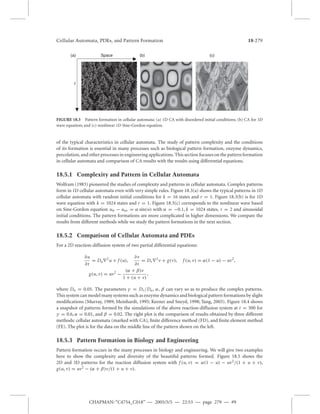
6. 18-276 Handbook of Bioinspired Algorithms and Applications
where u(x, y, t ) is the state variable that evolves with time in a 2D domain, and the function f (u) can be
either linear or nonlinear. D is a constant depending on the properties of diffusion. This equation can
also be considered as a vector form for a system of reaction-diffusion equations if let D = diag(D1,D2),
u = [u1u2]T. The discretization of this equation can be written as
un+1
i,j − un
i,j
1t = D
"
un
i+1,j − 2un
i,j + un
i−1,j
(1x)2 +
un
i,j+1 − 2un
i,j + un
i,j−1
(1y)2
#
+ f (un
i,j ),
by choosing 1t = 1x = 1y = 1, we have
un+1
i,j = D[un
i+1,j + un
i−1,j + un
i,j+1 + un
i,j−1] + f (un
i,j ) + (1 − 4D)un
i,j ,
which can be written as the generic form
ut+1
i,j =
Xr
k,l=−r
ak,lut
i+k,j+l + f (ut
i,j ),
where the summation is over the 4r + 1 neighborhood. This is a finite-state cellular automaton with the
coefficients ak,l being determined from the discretization of the governing equations, and for this special
case, we have a−1,0 = a+1,0 = a0,−1 = a0,+1 = D, a0,0 = 1 − 4D, r = 1.
18.3.4 Cellular Automata for the Wave Equation
For the 1D linear wave equation,
∂2u
∂t 2 = c2 ∂2u
∂x2 ,
where c is the wave speed. The simplest central difference scheme leads to
un+1
i − 2un
i + un−1
un
i
c2 (1t )2 = i+1 − 2un
i + un
i−1
(1x)2 .
By choosing 1t = 1x = 1, t = n, it becomes
ut+1
i = [ut
i ] − ut−1
i+1 + ut
i−1 + 2(1 − c2)ut
i .
This can be written in the generic form
ut+1
i + ut−1
i = g (ut ),
which is reversible under certain conditions. This property comes from the reversibility of the wave
equation because it is invariant under the transformation: t → −t .
18.3.5 Cellular Automata for Burgers Equation with Noise
One of the important equations arising in many processes such as turbulent phenomenon is the noisy
Burgers equation
∂u
∂t = 2u
∂u
∂x +
∂2u
∂x2 + ∇υ,
CHAPMAN: “C4754_C018” — 2005/5/5 — 22:53 — page 276 — #6

7. Cellular Automata, PDEs, and Pattern Formation 18-277
where υ is the noise that is uncorrelated in space and time so that hυ(x, t )i = 0 and hυ(x, t )υ(x0, t0)i =
CHAPMAN: “C4754_C018” — 2005/5/5 — 22:53 — page 277 — #7
AQ: Please check
Kahng has
changed to
Hahng
according to to
ref list.
2Dδ(x − x0)δ(t − t0) (Emmerich and Hahng, 1998). This equation with Gaussian white noise can be
rewritten as
∂u
∂t + ξ = 2u
∂u
∂x +
∂2u
∂x2 + η,
where both ξ and η are uncorrelated. By introducing the variables vt
i = c exp(1x ut
i ), φt
I = β ln(vt
i ),
α = 1t/(1x)2, (1 − 2α)/cα = exp(−A/β), c2 = exp(B/β), ξ = exp(8), η = exp(9) and after some
straightforward calculations in the limit of β tends zero, we have the automata rule
φt+1
i = φt
i−1 + max[0, φt
i − A, φt
i + φt
i+1 − B,9t
i − φt
i−1]
− max[0, φt
i−1 − A, φt
i−1 + φt
i − B,8ti
− φt
i−1],
where we have used the following identity,
lim
φ→+0
ε ln(eA/ε + eB/ε + · · · ) = max[A, B, . . .].
This forms a generalized probabilistic cellular automaton that is referred to as the noisy Burgers cellular
automaton. Burgers equation without noise usually evolves in shock wave, and in the presence of noise,
the states of the probabilistic cellular automata may be taken as discrete reminders of those shock waves
that were disorganized.
18.4 Differential Equations for Cellular Automata
Computer simulations based on cellular automata and partial differential equations work remarkably
well for many different reasons. One possibility is that finite-state cellular automata and finite difference
approximations using discrete time and space with a finite precision can represent physical variables
very well and thus the models are insensitive to very small space and time scales. It is relatively straight-forward
to derive the updating rules for cellular automata from the corresponding partial differential
equations. However, the reverse is usually very difficult. There is no generalmethod available to formulate
AQ: Please
specifyWolfram
1984a or b.
the continuum model or differential equations for given rule-based cellular automata despite the obvious
importance. Fortunately, there have been some important progress made in this area (Omohundro, 1984;
Wolfram, 1984), and we outline some of the procedures of formulating continuum equations for cellular
automata.
18.4.1 Formulation of Differential Equations from Cellular Automata
The mathematical analysis for cellular automata was first pioneered by Wolfram, and has attracted wide
attention since 1980s. Wolfram (1983) gave an extensive analysis of statistical mechanics of cellular
automata. Later on, Omohundro (1984) provided an instructive procedure of formulating the partial
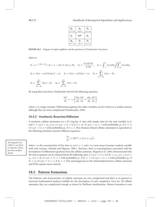
differential equations for cellular automata by using 10 PDE variables in 2D configurations. These ten
variables are the state variable P(x, y, t ) at present, new stateN(x, y, t ) and eight variablesU1, . . . ,U8 with
eight bump or bell functions. The eight variables have the same format of information as the P(x, y, t ).
On a 2D grid, these eight functions S1, . . . , S8 are shown in Figure 18.2 together with shifted coordinates.
According to Omohundro’s formulation, we assume the bumps to be α wide and constant outside β
AQ: Please check
if the change is
ok for paragraph
‘According to
Omohundro’s...’.
from the transition. If the width of a cell is 1, then α = 1/5 and β = 1/100. The eight functions are

8. 18-278 Handbook of Bioinspired Algorithms and Applications
S
2
S
3
S
4
(–1,+1) (0,+1) (+1,+1)
S
1 N/P
S
8
S
7
S
5
S
6
(–1,–1) (0,–1)
(+1,–1)
FIGURE 18.2 Diagram of eight neighbors and the positions of Omohundro’s functions.
CHAPMAN: “C4754_C018” — 2005/5/5 — 22:53 — page 278 — #8
taken as
S1 = e−1/(β−x)2
(−β < x < β), 0 (|x| ≥ β), S2 =
S1(xβ/α)
S1(0)
, S3 =
Z x
−1
S1(x)dx
ÁZ β
−β
S1(x)dx,
S4 = S3(x − α/2)S3(α/2 − x), S5 = S3(x − α)S3(α − x), S6 =
∞X
k=−∞
S4(x − k),
S7 =
∞X
k=−∞
S5(x − k), S8 =
∞X
k=−∞
S2(x − k).
By using these functions, Omohundro derived the following equation:
∂N
∂t = −γ
·
dS2
dx
∂N
∂x +
dS2
dy
∂N
∂y
¸
,
where γ is a large constant. Differential equations for other variables can be written in a similar manner
although they are more complicated (Omohundro, 1984).
18.4.2 Stochastic Reaction-Diffusion
A stochastic cellular automaton on a 1D ring has N sites with simple rules for the state variable ui (t )
and S = ui (t ) + ui+1(t ): (1) ui (t + 1) = 0, if S = 0; (2) ui (t + 1) = 1 with probability p1, if S = 1;
(3) ui (t + 1) = 1 with probability p2, if S = 2. This Domany–Kinzel cellular automaton is equivalent to
the following stochastic reaction-diffusion equation:
∂v
∂t = D∇2v + f (v) + ε√v,
where v is the concentration of live sites or ui (t ) = 1, and ε is a zero-mean Gaussian random variable
with unit variance (Ahmed and Elgazzar, 2001). However, there is nonuniqueness associated with the
formulation of differential equations from the cellular automata. Bognoli et al. (2002) demonstrated that
AQ: Bognoli et al.
(2002) is not listed
in reference. Please
provide complete
details.
the above equation can be obtained from the following rules: (1) ui (t +1) = 0, if 6 = ui+1(t )+ui (t )+
ui−1(t ) = 0; (2) ui (t + 1) = 1 with probability p1, if 6 = 1; (3) ui (t + 1) = 2 with probability p2, if
6 = 2; (4) ui (t + 1) = 1, if 6 = 3. This nonuniqueness in the relationship between cellular automata
and PDEs require more research.
18.5 Pattern Formation
The behavior and characteristics of cellular automata are very complicated and there is no general or
universal mathematical analysis available for the description of such complexity. Even for 1D cellular
automata, they are complicated enough as shown by Wolfram classifications. Pattern formation is one

9. Cellular Automata, PDEs, and Pattern Formation 18-279
(a) Space
(b) (c)
CHAPMAN: “C4754_C018” — 2005/5/5 — 22:53 — page 279 — #9
t
FIGURE 18.3 Pattern formation in cellular automata: (a) 1D CA with disordered initial conditions; (b) CA for 1D
wave equation; and (c) nonlinear 1D Sine-Gordon equation.
of the typical characteristics in cellular automata. The study of pattern complexity and the conditions
of its formation is essential in many processes such as biological pattern formation, enzyme dynamics,
percolation, and other processes in engineering applications. This section focuses on the pattern formation
in cellular automata and comparison of CA results with the results using differential equations.
18.5.1 Complexity and Pattern in Cellular Automata
Wolfram (1983) pioneered the studies of complexity and patterns in cellular automata. Complex patterns
form in 1D cellular automata even with very simple rules. Figure 18.3(a) shows the typical patterns in 1D
cellular automata with random initial conditions for k = 16 states and r = 1. Figure 18.3(b) is for 1D
wave equation with k = 1024 states and r = 1. Figure 18.3(c) corresponds to the nonlinear wave based
on Sine-Gordon equation utt − uxx = α sin(u) with α = −0.1, k = 1024 states, r = 2 and sinusoidal
initial conditions. The pattern formations are more complicated in higher dimensions. We compare the
results from different methods while we study the pattern formations in the next section.
18.5.2 Comparison of Cellular Automata and PDEs
For a 2D reaction-diffusion system of two partial differential equations:
∂u
∂t = Du∇2u + f (u),
∂v
∂t = Dv∇2v + g (v), f (u, v) = α(1 − u) − uv2,
g (u, v) = uv2 −
(α + β)v
1 + (u + v)
,
where Du = 0.05. The parameters γ = Dv/Du, α, β can vary so as to produce the complex patterns.
This systemcanmodelmany systems such as enzyme dynamics and biological pattern formations by slight
modifications (Murray, 1989; Meinhardt, 1995; Keener and Sneyd, 1998; Yang, 2003). Figure 18.4 shows
a snapshot of patterns formed by the simulations of the above reaction-diffusion system at t = 500 for
γ = 0.6, α = 0.01, and β = 0.02. The right plot is the comparison of results obtained by three different
methods: cellular automata (marked with CA), finite difference method (FD), and finite element method
(FE). The plot is for the data on the middle line of the pattern shown on the left.
18.5.3 Pattern Formation in Biology and Engineering
Pattern formation occurs in the many processes in biology and engineering. We will give two examples
here to show the complexity and diversity of the beautiful patterns formed. Figure 18.5 shows the
2D and 3D patterns for the reaction diffusion system with f (u, v) = α(1 − u) − uv2/(1 + u + v),
g (u, v) = uv2 − (α + β)v/(1 + u + v).

10. 18-280 Handbook of Bioinspired Algorithms and Applications
0.8
0.7
0.6
0.5
0.4
0.3
0.2
20 30 40 50 60 70 80
0.5
0.4
CHAPMAN: “C4754_C018” — 2005/5/5 — 22:53 — page 280 — #10
CA
FD
FE
100
90
80
70
60
50
40
30
20
10
20 40 60 80 100
0.6
0.55
0.45
0.35
0.3
FIGURE 18.4 A snapshot of pattern formation of the reaction-diffusion system (for α = 0.01, β = 0.02, and
γ = 0.6) and the comparison of results obtained by three different methods (CA, FD, FE) through the middle line of
the pattern on the left.
200
180
160
140
120
100
80
60
40
20
20 40 60 80 100 120 140 160 180 200
0.31
0.30
0.29
0.28
0.27
0.26
0.25
0.24
0.23
0.22
0.21
FIGURE 18.5 Pattern formations from 2D random initial conditions with α = 0.05, β = 0.01, and γ = 0.5 (left)
and 3D structures with α = 0.1, β = 0.05, and γ = 0.36 (right).
Another example is the formation of spiral waves studied by Barkley and his colleagues in detail (Barkley
et al., 1990;Margerit and Barkley, 2001)
∂u
∂t = ∇2u +
u
ε2
(1 − u)
µ
u −
v + β
α
¶
,
∂v
∂t = ε∇2v + (u − v),
where ε, α, β are parameters. Figure 18.6 shows the formation of spiral waves (2D) and scroll waves (3D)
of this nonlinear system under appropriate conditions.
AQ: Please identify
CA.
The patterns formed in terms of diffusion-reaction equations have been observed inmany phenomena.
The ring, spots, and stripes exist in animal skin coating, enzymatic reactions, shell structures, andmineral
formation. The spiral and scroll waves and spatiotemporal pattern formations are observed in calcium
transport, Belousov–Zhabotinsky reaction, cardiac tissue, and other excitable systems.
In this chapter, we have discussed some of important development and research results concerning the
connection among the cellular automata and partial differential equations as well as the pattern formation
related to both systems. Cellular automata are rule-based methods with the advantages of local inter-actions,
homogeneity, discrete states and parallelism, and thus they are suitable for simulating systems
with large degrees of freedom and life-related phenomena such as artificial intelligence and ecosystems.

11. Cellular Automata, PDEs, and Pattern Formation 18-281
FIGURE 18.6 Formation of spiral wave for α = 1, β = 0.1, and ε = 0.2 (left) and 3D scroll wave for α = 1, β = 0.1,
and ε = 0.15 (right).
PDEs are continuum-based models with the advantages of mathematical methods and closed-form
analytical solutions developed over many years, however, they usually deal with systems with small num-bers
of degree of freedom. There is an interesting connection between cellular automata and PDEs although
this is not always straightforward and sometimesmay be very difficult. The derivation of updating rules for
cellular automata from corresponding PDEs are relatively straightforward by using the finite differencing
schemes, while the formulation of differential equations from the cellular automaton is usually difficult
and nonunique. More studies are highly needed in these areas. In addition, either rule-based systems
or equation-based systems can have complex pattern formation under appropriate conditions, and these
spatiotemporal patterns can simulate many phenomena in engineering and biological applications.
References
Ahmed, E. and Elgazzar, A.S. On some applications of cellular automata. Physica A, 296 (2001) 529–538.
Barkley, D., Kness, M., and Tuckerman, L.S. Spiral-wave dynamics in a simple model of excitable media:
The transition from simple to compound rotation. Physical Review A, 42 (1990) 2489–2492.
Boffetta, G., Cencini, M., Falcioni, M., and Vulpiani, A. Predictability: A way to characterize complexity.
Physics Reports, 356 (2002) 367–474.
Cappuccio, R., Cattaneo, G., Erbacci, G., and Jocher, U. A parallel implementation of a cellular automata
based on the model for coffee percolation. Parallel Computing, 27 (2001) 685–717.
Emmerich, H. and Hahng, B.N. A random automata related to the noisy Burgers equation. Physica A, 259
(1998) 81–89.
CHAPMAN: “C4754_C018” — 2005/5/5 — 22:53 — page 281 — #11
AQ: Please
provide citation
for Boffetta et al.
(2002);
Cappuccio et al.
(2001); Flake
(1998);
Meinhardt
(1982); Turing
(1952);
von Newman
(1966) & Ostrov
and Rucker
(1996)
Flake, G.W. The Computational Beauty of Nature. MIT Press, Cambridge,MA (1998).
Guinot, V. Modelling using stochastic, finite state cellular automata: Rule inference from continuum
models. Applied Mathematical Modelling, 26 (2002) 701–714.
Keener, J. and Sneyd, J. Mathematical Physiology. Springer-Verlag, New York (1998).
Margolus, N. Physics-like models of computation. Physica D, 10 (1984) 81–95.
Margerit, D. and Barkley, D. Selection of twisted scroll waves in three-dimensional excitable media.
Physical Review Letters, 86 (2001) 175–178.
Meinhardt, H. Models of Biological Pattern Formation. Academic Press, London (1982).
Meinhardt, H. The Algorithmic Beauty of Sea Shells. Springer-Verlag, New York (1995).
Murray, J.D. Mathematical Biology. Springer-Verlag, New York (1989).
Omohundro, S. Modelling cellular automata with partial differential equations. Physica D, 10 (1984)
128–134.

12. 18-282 Handbook of Bioinspired Algorithms and Applications
Ostrov, D. and Rucker, R. Continuous-valued cellular automata for nonlinear wave equations. Complex
Systems, 10 (1996) 91–117.
Rucker, R. et al. CAPOW Software, www.mathcs.sjsu.edu/capow (1998).
CHAPMAN: “C4754_C018” — 2005/5/5 — 22:53 — page 282 — #12
AQ: Year has been
introduced from the
text for Rucker, R.
et al. Please check.
Toffoli, T. Cellular automata as an alternative to (rather than an approximate of) differential equations in
modelling physics. Physica D, 10 (1984) 117–127.
Turing, A. The chemical basis ofmorphogenesis. PhilosophicalTransactions of the Royal Society of London B,
237 (1952) 37–72.
Vichniac, G.Y. Simulating physics with cellular automata. Physica D, 10 (1984) 96–116.
von Newmann J. In A.W. Burks (Ed.), Theory of Self-Reproducing Automata. University of Illinois Press,
Urbana, IL (1966).
AQ: Please provide
the chapter title for
von Newman
(1966).
Weimar, J.R. Cellular automata for reaction-diffusion systems. Parallel Computing, 23 (1997) 1699–1715.
Wolfram, S. Statistical mechanics of cellular automata. Review of Modern Physics, 55 (1983) 601.
Wolfram, S. Cellular automata as models of complexity. Nature, 311 (1984a) 419–424.
Wolfram, S. Universality and complexity in cellular automata. Physica D, 10 (1984b) 1–35.
Wolfram, S. Cellular Automata and Complexity. Addison-Wesley, Reading, MA (1994).
Yang, X.S. Characterization of multispecies living ecosystems with cellular automata. In Standish, Abbass,
and Bedau (Eds.), Artificial Life VIII. MIT Press, Cambridge,MA (2002), pp. 138–141.
Yang, X.S. Turing pattern formation of catalytic reaction-diffusion systems in engineering applications.
Modelling and Simulation in Materials Science and Engineering, 11 (2003) 321–329.