This document summarizes a research paper that proposes a new metaheuristic optimization algorithm called Cuckoo Search (CS). CS is inspired by the breeding behavior of some cuckoo species. The paper describes the rules and steps of the CS algorithm, compares its performance to other algorithms on standard test functions and engineering design problems, and discusses unique features of CS like Lévy flights that make it promising for further research.

1. arXiv:1005.2908v3 [math.OC] 23 Dec 2010
Engineering Optimisation by Cuckoo Search
Xin-She Yang
Department of Engineering
University of Cambridge
Trumpington Street
Cambridge CB2 1PZ, UK
Suash Deb
Dept of Computer Science & Engineering
C. V. Raman College of Engineering
Bidyanagar, Mahura, Janla
Bhubaneswar 752054, INDIA
Abstract
A new metaheuristic optimisation algorithm, called Cuckoo Search (CS),
was developed recently by Yang and Deb (2009). This paper presents a more
extensive comparison study using some standard test functions and newly de-signed
stochastic test functions. We then apply the CS algorithm to solve
engineering design optimisation problems, including the design of springs and
welded beam structures. The optimal solutions obtained by CS are far better
than the best solutions obtained by an efficient particle swarm optimiser. We
will discuss the unique search features used in CS and the implications for fur-ther
research.
Reference to this paper should be made as follows:
Yang, X.-S., and Deb, S. (2010), “Engineering Optimisation by Cuckoo Search”,
Int. J. Mathematical Modelling and Numerical Optimisation, Vol. 1, No. 4,
330–343 (2010).
1 Introduction
Most design optimisation problems in engineering are often highly nonlinear, involv-ing
many different design variables under complex constraints. These constraints
can be written either as simple bounds such as the ranges of material properties,
or as nonlinear relationships including maximum stress, maximum deflection, mini-mum
load capacity, and geometrical configuration. Such nonlinearity often results in
multimodal response landscape. Subsequently, local search algorithms such as hill-climbing
and Nelder-Mead downhill simplex methods are not suitable, only global
algorithms should be used so as to obtain optimal solutions (Deb 1995, Arora 1989,
Yang 2005, Yang 2008).
Modern metaheuristic algorithms have been developed with an aim to carry out
global search, typical examples are genetic algorithms (Glodberg 1989), particle
swarm optimisation (PSO) (Kennedy and Eberhart 1995, Kennedy et al 2001). The
efficiency of metaheuristic algorithms can be attributed to the fact that they imitate
the best features in nature, especially the selection of the fittest in biological systems
which have evolved by natural selection over millions of years. Two important
characteristics of metaheuristics are: intensification and diversification (Blum and
Roli 2003, Gazi and Passino 2004, Yang 2009). Intensification intends to search
1

2. around the current best solutions and select the best candidates or solutions, while
diversification makes sure that the algorithm can explore the search space more
efficiently, often by randomization.
Recently, a new metaheuristic search algorithm, called Cuckoo Search (CS), has
been developed by Yang and Deb (2009). Preliminary studies show that it is very
promising and could outperform existing algorithms such as PSO. In this paper,
we will further study CS and validate it against test functions including stochastic
test functions. Then, we will apply it to solve design optimisation problems in
engineering. Finally, we will discuss the unique features of Cuckoo Search and
propose topics for further studies.
2 Cuckoo Search
In order to describe the Cuckoo Search more clearly, let us briefly review the inter-esting
breed behaviour of certain cuckoo species. Then, we will outline the basic
ideas and steps of the proposed algorithm.
2.1 Cuckoo Breeding Behaviour
Cuckoo are fascinating birds, not only because of the beautiful sounds they can
make, but also because of their aggressive reproduction strategy. Some species such
as the ani and Guira cuckoos lay their eggs in communal nests, though they may
remove others’ eggs to increase the hatching probability of their own eggs (Payne et
al 2005). Quite a number of species engage the obligate brood parasitism by laying
their eggs in the nests of other host birds (often other species). There are three basic
types of brood parasitism: intraspecific brood parasitism, cooperative breeding, and
nest takeover. Some host birds can engage direct conflict with the intruding cuckoos.
If a host bird discovers the eggs are not its owns, it will either throw these alien eggs
away or simply abandons its nest and builds a new nest elsewhere. Some cuckoo
species such as the New World brood-parasitic Tapera have evolved in such a way
that female parasitic cuckoos are often very specialized in the mimicry in colour and
pattern of the eggs of a few chosen host species (Payne et al 2005). This reduces the
probability of their eggs being abandoned and thus increases their reproductivity.
Furthermore, the timing of egg-laying of some species is also amazing. Parasitic
cuckoos often choose a nest where the host bird just laid its own eggs. In general, the
cuckoo eggs hatch slightly earlier than their host eggs. Once the first cuckoo chick
is hatched, the first instinct action it will take is to evict the host eggs by blindly
propelling the eggs out of the nest, which increases the cuckoo chick’s share of food
provided by its host bird (Payne et al 2005). Studies also show that a cuckoo chick
can also mimic the call of host chicks to gain access to more feeding opportunity.
2.2 L´evy Flights
In nature, animals search for food in a random or quasi-random manner. In general,
the foraging path of an animal is effectively a random walk because the next move
is based on the current location/state and the transition probability to the next
location. Which direction it chooses depends implicitly on a probability which can
be modelled mathematically. For example, various studies have shown that the flight
2

3. behaviour of many animals and insects has demonstrated the typical characteristics
of L´evy flights (Brown et al 2007, Reynods and Frye 2007, Pavlyukevich 2007).
A recent study by Reynolds and Frye (2007) shows that fruit flies or Drosophila
melanogaster, explore their landscape using a series of straight flight paths punc-tuated
by a sudden 90o turn, leading to a L´evy-flight-style intermittent scale-free
search pattern. Studies on human behaviour such as the Ju/’hoansi hunter-gatherer
foraging patterns also show the typical feature of L´evy flights. Even light can be
related to L´evy flights (Barthelemy et al 2008). Subsequently, such behaviour has
been applied to optimization and optimal search, and preliminary results show its
promising capability (Shlesinger 2006, Pavlyukevich 2007).
2.3 Cuckoo Search
For simplicity in describing our new Cuckoo Search (Yang and Deb 2009), we now
use the following three idealized rules:
• Each cuckoo lays one egg at a time, and dumps it in a randomly chosen nest;
• The best nests with high quality of eggs (solutions) will carry over to the next
generations;
• The number of available host nests is fixed, and a host can discover an alien
egg with a probability pa ∈ [0, 1]. In this case, the host bird can either throw
the egg away or abandon the nest so as to build a completely new nest in a
new location.
For simplicity, this last assumption can be approximated by a fraction pa of the
n nests being replaced by new nests (with new random solutions at new locations).
For a maximization problem, the quality or fitness of a solution can simply be
proportional to the objective function. Other forms of fitness can be defined in a
similar way to the fitness function in genetic algorithms.
Based on these three rules, the basic steps of the Cuckoo Search (CS) can be
summarised as the pseudo code shown in Fig. 1.
When generating new solutions x(t+1) for, say cuckoo i, a L´evy flight is performed
x
(t+1)
i = x
(t)
i + α ⊕ L´evy(λ), (1)
where α > 0 is the step size which should be related to the scales of the problem
of interest. In most cases, we can use α = O(1). The product ⊕ means entry-wise
multiplications. L´evy flights essentially provide a random walk while their random
steps are drawn from a L´evy distribution for large steps
L´evy ∼ u = t−λ, (1 < λ ≤ 3), (2)
which has an infinite variance with an infinitemean. Here the consecutive jumps/steps
of a cuckoo essentially form a random walk process which obeys a power-law step-length
distribution with a heavy tail.
It is worth pointing out that, in the real world, if a cuckoo’s egg is very similar
to a host’s eggs, then this cuckoo’s egg is less likely to be discovered, thus the fitness
should be related to the difference in solutions. Therefore, it is a good idea to do
a random walk in a biased way with some random step sizes. A demo version is
attached in the Appendix (this demo is not published in the actual paper, but as a
supplement to help readers to implement the cuckoo search correctly).
3

4. Objective function f(x), x = (x1, ..., xd)T ;
Initial a population of n host nests xi (i = 1, 2, ..., n);
while (t <MaxGeneration) or (stop criterion);
Get a cuckoo (say i) randomly by L´evy flights;
Evaluate its quality/fitness Fi;
Choose a nest among n (say j) randomly;
if (Fi > Fj),
Replace j by the new solution;
end
Abandon a fraction (pa) of worse nests
[and build new ones at new locations via L´evy flights];
Keep the best solutions (or nests with quality solutions);
Rank the solutions and find the current best;
end while
Postprocess results and visualisation;
Figure 1: Cuckoo Search (CS).
3 Implementation and Validation
3.1 Validation and Parameter Studies
It is relatively easy to implement the algorithm, and then we have to benchmark it
using test functions with analytical or known solutions. There are many benchmark
test functions and there is no standard list or collection, though extensive descrip-tions
of various functions do exist in literature (Floudas et al 1999, Hedar 2005,
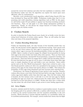
Molga and Smutnicki 2005). For example, Michalewicz’s test function has many
local optima
f(x) = −
Xd
i=1
h
sin(
sin(xi)
ix2i π
i2m
)
, (m = 10), (3)
in the domain 0 ≤ xi ≤ π for i = 1, 2, ..., d where d is the number of dimensions.
The global mimimum f
≈ −1.801 occurs at (2.20319, 1.57049) for d = 2, while
f
≈ −4.6877 for d = 5. In the 2D case, its 3D landscape is shown Fig. 2.
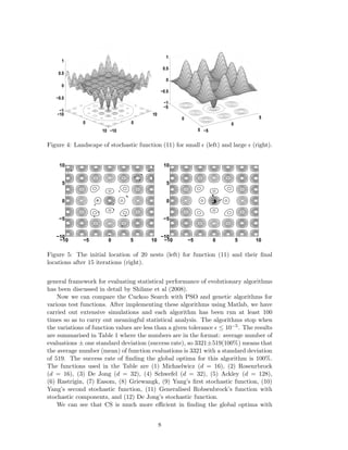
The global optimum in 2D can easily be found using Cuckoo Search, and the
results are shown in Fig. 3 where the final locations of the nests are marked with
⋄. Here we have used n = 20 nests, α = 1 and pa = 0.25. From the figure, we can
see that, as the optimum is approaching, most nests aggregate towards the global
optimum. In various simulations, we also notice that nests are also distributed at
different (local) optima in the case of multimodal functions. This means that CS
can find all the optima simultaneously if the number of nests are much higher than
the number of local optima. This advantage may become more significant when
dealing with multimodal and multiobjective optimization problems.
We have also tried to vary the number of host nests (or the population size n)
and the probability pa. We have used n = 5, 10, 15, 20, 50, 100, 150, 250, 500 and
pa = 0, 0.01, 0.05, 0.1, 0.15, 0.2, 0.25, 0.4, 0.5. From our simulations, we found that
n = 15 to 25 and pa = 0.15 to 0.30 are sufficient for most optimization problems.
4

5. 2
1
0
−1
0
2
4
6 0
2
4
6
−2
Figure 2: The landscape of Michaelwicz’s 2D function.
Results and analysis also imply that the convergence rate, to some extent, is not
sensitive to the parameters used. This means that the fine adjustment of algorithm-dependent
parameters is not needed for any given problems. Therefore, we will use
n = 20 and pa = 0.25 in the rest of the simulations, especially for the comparison
studies presented later.
3.2 Standard Test Functions
Various test functions in literature are designed to test the performance of optimiza-tion
algorithms (Chattopadhyay 1971, Schoen 1993, Shang and Qiu 2006). Any new
optimization algorithm should also be validated and tested against these benchmark
functions. In our simulations, we have used the following test functions.
De Jong’s first function is essentially a sphere function
f(x) =
Xd
i=1
x2i
, xi ∈ [−5.12, 5.12], (4)
whose global minimum f(x
) = 0 occurs at x
= (0, 0, ..., 0). Here d is the dimen-sion.
The generalized Rosenbrock’s function is given by
f(x) =
dX−1
i=1
h
(1 − xi)2 + 100(xi+1 − x2i
)2
i
, (5)
which has a unique global minimum f
= 0 at x
= (1, 1, ..., 1).
5

6. 5
4
3
2
1
0
0 1 2 3 4 5
5
4
3
2
1
0
0 1 2 3 4 5
Figure 3: Initial locations of 20 nests in Cuckoo Search, and their final locations are
marked with ⋄.
Schwefel’s test function is multimodal
f(x) =
Xd
i=1
q
|xi| )
h
− xi sin(
i
, −500 ≤ xi ≤ 500, (6)
whose global minimum f
= −418.9829d is at xi
= 420.9687(i = 1, 2, ..., d).
Ackley’s function is also multimodal
f(x) = −20 exp
vuut
− 0.2
1
d
Xd
i=1
x2i
#
− exp[
1
d
Xd
i=1
cos(2πxi)] + (20 + e), (7)
with the global minimum f
= 0 at x
= (0, 0, ..., 0) in the range of −32.768 ≤ xi ≤
32.768 where i = 1, 2, ..., d.
Rastrigin’s test function
f(x) = 10d +
Xd
i=1
[x2i − 10 cos(2πxi)], (8)
has a unique global minimum f
= 0 at (0, 0, ..., 0) in a hypercube −5.12 ≤ xi ≤ 5.12
where i = 1, 2, ..., d.
Easom’s test function has a sharp tip
f(x, y) = −cos(x) cos(y) exp[−(x − π)2 − (y − π)2], (9)
in the domain (x, y) ∈ [−100, 100]×[−100, 100]. It has a global minimum of f
= −1
at (π, π) in a very small region.
Griewangk’s test function has many local minima
f(x) =
1
4000
Xd
i=1
x2i
−
Yd
i=1
cos(
xi √i
) + 1, (10)
but a unique global mimimum f
= 0 at (0, 0, ..., 0) for all −600 ≤ xi ≤ 600 where
i = 1, 2, ..., d.
6

7. 3.3 Stochastic Test Functions
Almost all the test functions in literature are deterministic. It is usually more
difficult for algorithms to deal with stochastic functions. We have designed some
stochastic test functions for such a purpose.
The first test function designed by Yang (2010) looks like a standing-wave func-tion
with a region of defects
f(x) =
h
e−
Pd
2m
− 2e−
i=1(xi/)¯
Pd
i=1 ǫi(xi−π)2i
·
Yd
i=1
cos2 xi, m = 5, (11)
which has many local minima and the unique global minimum f
= −1 at x
=
(π, π, ..., π) for =¯
15 within the domain −20 ≤ xi ≤ 20 for i = 1, 2, ..., d. Here the
random variables ǫi (i = 1, 2, ..., d) are uniformly distributed in (0, 1). For example,
if all ǫi are relatively small (say order of 0.05), a snapshot of the landscape in 2D is
shown in Fig. 4, while for higher values such as 0.5 the landscape is different, also
shown in Fig. 4.
Yang’s second test function is also multimodal but it has a singularity
f(x) =
Xd
i=1
exp
ǫi|xi|
h
−
Xd
i=1
sin(x2i
i
, (12)
)
which has a unique global minimum f
= 0 at x
= (0, 0, ..., 0) in the domain
−2π ≤ xi ≤ 2π where i = 1, 2, ..., d (Yang 2010). This function is singular at the
optimum (0, ..., 0). Similarly, ǫi should be drawn from a uniform distribution in [0, 1]
or Unif[0,1]. In fact, using the same methodology, we can turn many determistic
functions into stochastic test functions. For example, we can extend Robsenbrock’s
function as the following stochastic function
f(x) =
dX−1
i=1
h
(1 − xi)2 + 100ǫi(xi+1 − x2i
)2
i
, (13)
where ǫi should be drawn from Unif[0,1]. Similarly, we can also extend De Jong’s
function into its corresponding stochastic form
f(x) =
Xd
i=1
ǫix2i
, (14)
which still has the same global minimum f
= 0 at (0, 0, ..., 0), despite its stochastic
nature due to the factor ǫi. For stochastic functions, most deterministic algorithms
such as hill climbing and Nelder-Mead downhill simplex method would simply fail.
However, we can see later that most metaheuristic algorithms such as PSO and CS
are still robust.
3.4 Simulations and Comparison
Recent studies indicate that PSO can outperform genetic algorithms (GA) and other
conventional algorithms (Goldberg 1989, Kennedy et al 2001, Yang 2008). This can
be attributed partly to the broadcasting ability of the current best estimates, po-tentially
leading to a better and quicker convergence rate towards the optimality. A
7

8. 1
0.5
0
−0.5
−10
0
10 −10
0
10
−1
1
0.5
0
−0.5
−5
0
5 −5
0
5
−1
Figure 4: Landscape of stochastic function (11) for small ǫ (left) and large ǫ (right).
10
5
0
−5
−10
−10 −5 0 5 10
10
5
0
−5
−10
−10 −5 0 5 10
Figure 5: The initial location of 20 nests (left) for function (11) and their final
locations after 15 iterations (right).
general framework for evaluating statistical performance of evolutionary algorithms
has been discussed in detail by Shilane et al (2008).
Now we can compare the Cuckoo Search with PSO and genetic algorithms for
various test functions. After implementing these algorithms using Matlab, we have
carried out extensive simulations and each algorithm has been run at least 100
times so as to carry out meaningful statistical analysis. The algorithms stop when
the variations of function values are less than a given tolerance ǫ ≤ 10−5. The results
are summarised in Table 1 where the numbers are in the format: average number of
evaluations ± one standard deviation (success rate), so 3321±519(100%) means that
the average number (mean) of function evaluations is 3321 with a standard deviation
of 519. The success rate of finding the global optima for this algorithm is 100%.
The functions used in the Table are (1) Michaelwicz (d = 16), (2) Rosenrbrock
(d = 16), (3) De Jong (d = 32), (4) Schwefel (d = 32), (5) Ackley (d = 128),
(6) Rastrigin, (7) Easom, (8) Griewangk, (9) Yang’s first stochastic function, (10)
Yang’s second stochastic function, (11) Generalised Robsenbrock’s function with
stochastic components, and (12) De Jong’s stochastic function.
We can see that CS is much more efficient in finding the global optima with
8

9. Table 1: Comparison of CS with genetic algorithms and particle swarm optimisation
Functions GA PSO CS
(1) 89325 ± 7914(95%) 6922 ± 537(98%) 3221 ± 519(100%)
(2) 55723 ± 8901(90%) 32756 ± 5325(98%) 5923 ± 1937(100%)
(3) 15232 ± 1270(100%) 10079 ± 970(100%) 3015 ± 540(100%)
(4) 23790 ± 6523(95%) 92411 ± 1163(97%) 4710 ± 592(100%)
(5) 32720 ± 3327(90%) 23407 ± 4325(92%) 4936 ± 903(100%)
(6) 110523 ± 5199(77%) 79491 ± 3715(90%) 10354 ± 3755(100%)
(7) 19239 ± 3307(92%) 17273 ± 2929(90%) 6751 ± 1902(100%)
(8) 70925 ± 7652(90%) 55970 ± 4223(92%) 10912 ± 4050(100%)
(9) 79025 ± 6312(49%) 34056 ± 4470(90%) 11254 ± 2733(99%)
(10) 35072 ± 3730(54%) 22360 ± 2649(92%) 8669 ± 3480(98%)
(11) 63268 ± 5091(40%) 49152 ± 6505(89%) 10564 ± 4297(99%)
(12) 24164 ± 4923(68%) 11780 ± 4912(94%) 7723 ± 2504(100%)
higher success rates. Each function evaluation is virtually instantaneous on a modern
personal computer. For example, the computing time for 10,000 evaluations on a
3GHz desktop is about 5 seconds. In addition, for stochastic functions, genetic
algorithms do not perform well, while PSO is better. However, CS is far more
promising.
4 Engineering Design
Design optimisation is an integrated part of designing any new products in engineer-ing
and industry. Most design problems are complex and multiobjective, sometimes
even the optimal solutions of interest do not exist. In order to see how the CS
algorithm may perform, we now use two standard but well-known test problems.
4.1 Spring Design Optimisation
Tensional and/or compressional springs are used widely in engineering. A standard
spring design problem has three design variables: the wire diameter w, the mean
coil diameter d, and the length (or number of coils) L.
The objective is to minimise the weight of the spring, subject to various con-straints
such as maximum shear stress, minimum deflection, and geometrical limits.
For detailed description, please refer to earlier studies (Belegundu 1982, Arora 1989,
Cagnina et al 2008). This problem can be written compactly as
Minimise f(x) = (L + 2)w2d, (15)
9

10. subject to
g1(x) = 1 − d3L
71785w4 ≤ 0,
g2(x) = 1 − 140.45w
d2L ≤ 0,
g3(x) = 2(w+d)
3 − 1 ≤ 0,
g4(x) = d(4d−w)
w3(12566d−w) + 1
5108w2 − 1 ≤ 0,
(16)
with the following limits
0.05 ≤ w ≤ 2.0, 0.25 ≤ d ≤ 1.3, 2.0 ≤ L ≤ 15.0. (17)
Using Cuckoo Search, we have obtained the same or slightly better solutions
than the best solution obtained by Cagnina et al (2008)
f
= 0.012665 at (0.051690, 0.356750, 11.287126), (18)
but cuckoo search uses significantly fewer evaluations.
4.2 Welded Beam Design
The so-called welded beam design is another standard test problem for constrained
design optimisation (Ragsdell and Phillips 1976, Cagnina et al 2008). The problem
has four design variables: the width w and length L of the welded area, the depth
h and thickness h of the main beam. The objective is to minimise the overall
fabrication cost, under the appropriate constraints of shear stress τ , bending stress
σ, buckling load P and maximum end deflection δ.
The problem can be written as
minimise f(x) = 1.10471w2L + 0.04811dh(14.0 + L), (19)
subject to
g1(x) = w − h ≤ 0,
g2(x) = δ(x) − 0.25 ≤ 0,
g3(x) = τ (x) − 13, 600 ≤ 0,
g4(x) = σ(x) − 30, 000 ≤ 0,
g5(x) = 0.10471w2 + 0.04811hd(14 + L) − 5.0 ≤ 0,
g6(x) = 0.125 − w ≤ 0,
g7(x) = 6000 − P(x) ≤ 0,
(20)
10

11. where
σ(x) = 504,000
hd2 , Q = 6000(14 + L
2 ),
D = 1
2
p
L2 + (w + d)2, J = √2 wL[L2
6 + (w+d)2
2 ],
30,000hd3 , β = QD
δ = 65,856
J ,
α = 6000
p2wL
, τ (x) =
q
α2 + αβL
D + β2,
P = 0.61423 × 106 dh3
6 (1 −
d√30/48
28 ).
(21)
The simple limits or bounds are 0.1 ≤ L, d ≤ 10 and 0.1 ≤ w, h ≤ 2.0.
Using our Cuckoo Search, we have the following optimal solution
x
= (w,L, d, h)
= (0.205729639786079, 3.470488665627977, 9.036623910357633, 0.205729639786079),
(22)
with
f(x∗)min = 1.724852308597361. (23)
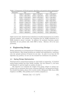
This solution is exactly the same as the solution obtained by Cagnina et al (2008)
f
= 1.724852 at (0.205730, 3.470489, 9.036624, 0.205729). (24)
We have seen that, for both test problems, CS has found the optimal solutions which
are either better than or the same as the solutions found so far in literature.
5 Discussions and Conclusions
From the comparison study of the performance of CS with GAs and PSO, we know
that our new Cuckoo Search in combination with L´evy flights is very efficient and
proves to be superior for almost all the test problems. This is partly due to the fact
that there are fewer parameters to be fine-tuned in CS than in PSO and genetic algo-rithms.
In fact, apart from the population size n, there is essentially one parameter
pa. If we look at the CS algorithm carefully, there are essentially three compo-nents:
selection of the best, exploitation by local random walk, and exploration by
randomization via L´evy flights globally.
The selection of the best by keeping the best nests or solutions is equivalent
to some form of elitism commonly used in genetic algorithms, which ensures the
best solution is passed onto the next iteration and there is no risk that the best
solutions are cast out of the population. The exploitation around the best solutions
is performed by using a local random walk
x
t+1 = x
t + αt. (25)
If t obeys a Gaussian distribution, this becomes a standard random walk indeed.
This is equivalent to the crucial step in pitch adjustment in Harmony Search (Geem
11

12. et al 2001, Yang 2009). If t is drawn from a L´evy distribution, the step of move
is larger, and could be potentially more efficient. However, if the step is too large,
there is risk that the move is too far away. Fortunately, the elitism by keeping the
best solutions makes sure that the exploitation moves are within the neighbourhood
of the best solutions locally.
On the other hand, in order to sample the search space effectively so that new
solutions to be generated are diverse enough, the exploration step is carried out in
terms of L´evy flights. In contrast, most metaheuristic algorithms use either uniform
distributions or Gaussian to generate new explorative moves (Geem et al 2001, Blum
and Rilo 2003). If the search space is large, L´evy flights are usually more efficient.
A good combination of the above three components can thus lead to an efficient
algorithm such as Cuckoo Search.
Furthermore, our simulations also indicate that the convergence rate is insensi-tive
to the algorithm-dependent parameters such as pa. This also means that we
do not have to fine tune these parameters for a specific problem. Subsequently, CS
is more generic and robust for many optimisation problems, comparing with other
metaheuristic algorithms.
This potentially powerful optimisation strategy can easily be extended to study
multiobjecitve optimization applications with various constraints, including NP-hard
problems. Further studies can focus on the sensitivity and parameter studies
and their possible relationships with the convergence rate of the algorithm. In
addition, hybridization with other popular algorithms such as PSO will also be
potentially fruitful. More importantly, as for most metaheuristic algorithms, math-ematical
analysis of the algorithm structures is highly needed. At the moment, no
such framework exists for analyzing metaheuristics in general. Any progress in this
area will potentially provide new insight into the understanding of how and why
metaheuristic algorithms work.
References
[1] Arora, J., 1989. Introduction to Optimum Design, McGraw-Hill.
[2] Belegundu, A., 1982. ‘A study of mathematical programming methods for
structural optimization’, PhD thesis, Department of Civil Environmental En-gineering,
University of Iowa, USA.
[3] Barthelemy, P., Bertolotti, J., Wiersma, D. S., 2008. ‘A L´evy flight for light’,
Nature, 453, 495-498.
[4] Blum, C. and Roli, A., 2003. ‘Metaheuristics in combinatorial optimization:
Overview and conceptural comparision’, ACM Comput. Surv., 35, 268-308.
[5] Brown, C., Liebovitch, L. S., Glendon, R., 2007. ‘L´evy flights in Dobe
Ju/’hoansi foraging patterns’, Human Ecol., 35, 129-138.
[6] Cagnina, L. C., Esquivel, S. C., and Coello, C. A., 2008. ‘Solving engineering
optimization problems with the simple constrained particle swarm optimizer’,
Informatica, 32, 319-326.
12

13. [7] Chattopadhyay, R., 1971. ‘A study of test functions for optimization algo-rithms’,
J. Opt. Theory Appl., 8, 231-236.
[8] Deb, K., 1995. Optimisation for Engineering Design, Prentice-Hall, New Delhi.
[9] Floudas, C. A., Pardalos, P. M., Adjiman, C. S., Esposito, W. R., Gumus,
Z. H., Harding, S. T., Klepeis, J. L., Meyer, C. A., Scheiger, C. A., 1999.
Handbook of Test Problems in Local and Global Optimization, Springer, 1999.
[10] Gazi, K., and Passino, K.M., 2004. Stability analysis of social foraging swarms,
IEEE Trans. Sys. Man. Cyber. Part B - Cybernetics, 34, 539-557.
[11] Geem, Z. W., Kim, J. H., Loganathan, G. V., 2001. ‘A new heuristic opti-mization
algorithm: Harmony search’, Simulation, 76, 60-68.
[12] Goldberg, D. E., 1989. Genetic Algorithms in Search, Optimisation and Ma-chine
Learning, Reading, Mass., Addison Wesley.
[13] Hedar, A., 2005, ‘Test function web pages’,
http://www-optima.amp.i.kyoto-u.ac.jp /member/student/hedar/Hedar files/TestGO files/Page364.htm
[14] Kennedy, J. and Eberhart, R. C., 1995. ‘Particle swarm optimization’. Proc.
of IEEE International Conference on Neural Networks, Piscataway, NJ. pp.
1942-1948.
[15] Kennedy, J., Eberhart, R. C., Shi, Y., 2001. Swarm intelligence, Academic
Press.
[16] Molga, M., Smutnicki, C., 2005. “Test functions for optimization needs”,
http://www.zsd.ict.pwr.wroc.pl/files/docs/functions.pdf
[17] Passino, K. M., 2001. Biomimicry of Bacterial Foraging for Distributed Opti-mization,
University Press, Princeton, New Jersey.
[18] Payne, R. B., Sorenson, M. D., and Klitz, K.,2005. The Cuckoos, Oxford
University Press.
[19] Pavlyukevich, I., 2007. ‘L´evy flights, non-local search and simulated anneal-ing’,
J. Computational Physics, 226, 1830-1844.
[20] Ragsdell, K. and Phillips, D.,1976. ‘Optimal design of a class of welded struc-tures
using geometric programming’, J. Eng. Ind., 98, 1021-1025.
[21] Reynolds, A. M. and Frye, M. A., 2007. ‘Free-flight odor tracking in Drosophila
is consistent with an optimal intermittent scale-free search’, PLoS One, 2,
e354.
[22] Schoen, F., 1993. ‘A wide class of test functions for global optimization’, J.
Global Optimization, 3, 133-137.
[23] Shang, Y. W., Qiu Y. H., 2006. ‘A note on the extended rosenrbock function’,
Evolutionary Computation, 14, 119-126.
13

14. [24] Shilane D., Martikainen J., Dudoit S., Ovaska S. J., 2008. ‘A general frame-work
for statistical performance comparison of evolutionary computation al-gorithms’,
Information Sciences, 178, 2870-2879.
[25] Shlesinger, M. F.,2006. ‘Search research’, Nature, 443, 281-282.
[26] Yang, X. S., 2008. Nature-Inspired Metaheuristic Algorithms, Luniver Press,
(2008).
[27] Yang, X. S., 2005. ‘Biology-derived algorithms in engineering optimizaton’
(chapter 32), in Handbook of Bioinspired Algorithms and Applications (eds
Olarius Zomaya), Chapman Hall / CRC.
[28] Yang, X. S. and Deb, S., 2009. ‘Cuckoo search via L´evy flights’, Proceeings of
World Congress on Nature Biologically Inspired Computing (NaBIC 2009,
India), IEEE Publications, USA, pp. 210-214.
[29] Yang, X. S., 2009. ‘Harmony search as a metaheuristic algorithm’, in: Music-
Inspired Harmony Search: Theory and Applications (Eds Z. W. Geem),
Springer, pp.1-14.
[30] Yang, X. S., 2010. Engineering Optimisation: An Introduction with Meta-heuristic
Applications, John Wiley and Sons.
Appendix: Demo Implementation
% -----------------------------------------------------------------
% Cuckoo Search (CS) algorithm by Xin-She Yang and Suash Deb %
% Programmed by Xin-She Yang at Cambridge University %
% Programming dates: Nov 2008 to June 2009 %
% Last revised: Dec 2009 (simplified version for demo only) %
% -----------------------------------------------------------------
% Papers -- Citation Details:
% 1) X.-S. Yang, S. Deb, Cuckoo search via Levy flights,
% in: Proc. of World Congress on Nature Biologically Inspired
% Computing (NaBIC 2009), December 2009, India,
% IEEE Publications, USA, pp. 210-214 (2009).
% http://arxiv.org/PS_cache/arxiv/pdf/1003/1003.1594v1.pdf
% 2) X.-S. Yang, S. Deb, Engineering optimization by cuckoo search,
% Int. J. Mathematical Modelling and Numerical Optimisation,
% Vol. 1, No. 4, 330-343 (2010).
% http://arxiv.org/PS_cache/arxiv/pdf/1005/1005.2908v2.pdf
% ----------------------------------------------------------------%
% This demo program only implements a standard version of %
% Cuckoo Search (CS), as the Levy flights and generation of %
% new solutions may use slightly different methods. %
% The pseudo code was given sequentially (select a cuckoo etc), %
% but the implementation here uses Matlab’s vector capability, %
% which results in neater/better codes and shorter running time. %
% This implementation is different and more efficient than the %
% the demo code provided in the book by
% Yang X. S., Nature-Inspired Metaheuristic Algoirthms, %
% 2nd Edition, Luniver Press, (2010). %
14

15. % --------------------------------------------------------------- %
% =============================================================== %
% Notes: %
% Different implementations may lead to slightly different %
% behavour and/or results, but there is nothing wrong with it, %
% as this is the nature of random walks and all metaheuristics. %
% -----------------------------------------------------------------
function [bestnest,fmin]=cuckoo_search(n)
if nargin1,
% Number of nests (or different solutions)
n=25;
end
% Discovery rate of alien eggs/solutions
pa=0.25;
%% Change this if you want to get better results
% Tolerance
Tol=1.0e-5;
%% Simple bounds of the search domain
% Lower bounds
nd=15;
Lb=-5*ones(1,nd);
% Upper bounds
Ub=5*ones(1,nd);
% Random initial solutions
for i=1:n,
nest(i,:)=Lb+(Ub-Lb).*rand(size(Lb));
end
% Get the current best
fitness=10^10*ones(n,1);
[fmin,bestnest,nest,fitness]=get_best_nest(nest,nest,fitness);
N_iter=0;
%% Starting iterations
while (fminTol),
% Generate new solutions (but keep the current best)
new_nest=get_cuckoos(nest,bestnest,Lb,Ub);
[fnew,best,nest,fitness]=get_best_nest(nest,new_nest,fitness);
% Update the counter
N_iter=N_iter+n;
% Discovery and randomization
new_nest=empty_nests(nest,Lb,Ub,pa) ;
% Evaluate this set of solutions
[fnew,best,nest,fitness]=get_best_nest(nest,new_nest,fitness);
% Update the counter again
N_iter=N_iter+n;
% Find the best objective so far
15

16. if fnewfmin,
fmin=fnew;
bestnest=best;
end
end %% End of iterations
%% Post-optimization processing
%% Display all the nests
disp(strcat(’Total number of iterations=’,num2str(N_iter)));
fmin
bestnest
%% --------------- All subfunctions are list below ------------------
%% Get cuckoos by ramdom walk
function nest=get_cuckoos(nest,best,Lb,Ub)
% Levy flights
n=size(nest,1);
% Levy exponent and coefficient
% For details, see equation (2.21), Page 16 (chapter 2) of the book
% X. S. Yang, Nature-Inspired Metaheuristic Algorithms, 2nd Edition, Luniver Press, (2010).
beta=3/2;
sigma=(gamma(1+beta)*sin(pi*beta/2)/(gamma((1+beta)/2)*beta*2^((beta-1)/2)))^(1/beta);
for j=1:n,
s=nest(j,:);
% This is a simple way of implementing Levy flights
% For standard random walks, use step=1;
%% Levy flights by Mantegna’s algorithm
u=randn(size(s))*sigma;
v=randn(size(s));
step=u./abs(v).^(1/beta);
% In the next equation, the difference factor (s-best) means that
% when the solution is the best solution, it remains unchanged.
stepsize=0.01*step.*(s-best);
% Here the factor 0.01 comes from the fact that L/100 should the typical
% step size of walks/flights where L is the typical lenghtscale;
% otherwise, Levy flights may become too aggresive/efficient,
% which makes new solutions (even) jump out side of the design domain
% (and thus wasting evaluations).
% Now the actual random walks or flights
s=s+stepsize.*randn(size(s));
% Apply simple bounds/limits
nest(j,:)=simplebounds(s,Lb,Ub);
end
%% Find the current best nest
function [fmin,best,nest,fitness]=get_best_nest(nest,newnest,fitness)
% Evaluating all new solutions
for j=1:size(nest,1),
fnew=fobj(newnest(j,:));
if fnew=fitness(j),
fitness(j)=fnew;
nest(j,:)=newnest(j,:);
16

17. end
end
% Find the current best
[fmin,K]=min(fitness) ;
best=nest(K,:);
%% Replace some nests by constructing new solutions/nests
function new_nest=empty_nests(nest,Lb,Ub,pa)
% A fraction of worse nests are discovered with a probability pa
n=size(nest,1);
% Discovered or not -- a status vector
K=rand(size(nest))pa;
% In the real world, if a cuckoo’s egg is very similar to a host’s eggs, then
% this cuckoo’s egg is less likely to be discovered, thus the fitness should
% be related to the difference in solutions. Therefore, it is a good idea
% to do a random walk in a biased way with some random step sizes.
%% New solution by biased/selective random walks
stepsize=rand*(nest(randperm(n),:)-nest(randperm(n),:));
new_nest=nest+stepsize.*K;
% Application of simple constraints
function s=simplebounds(s,Lb,Ub)
% Apply the lower bound
ns_tmp=s;
I=ns_tmpLb;
ns_tmp(I)=Lb(I);
% Apply the upper bounds
J=ns_tmpUb;
ns_tmp(J)=Ub(J);
% Update this new move
s=ns_tmp;
%% You can replace the following by your own functions
% A d-dimensional objective function
function z=fobj(u)
%% d-dimensional sphere function sum_j=1^d (u_j-1)^2.
% with a minimum at (1,1, ...., 1);
z=sum((u-1).^2);
17