138191 rvsp lecture notes

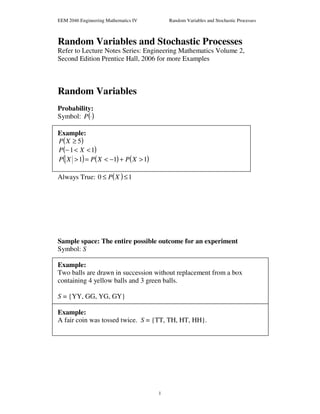
EEM 2046 Engineering Mathematics IV Random Variables and Stochastic Processes
1
Random Variables and Stochastic Processes
Refer to Lecture Notes Series: Engineering Mathematics Volume 2,
Second Edition Prentice Hall, 2006 for more Examples
Random Variables
Probability:
Symbol: ( )⋅P
Example:
( )5≥XP
( )11 <<− XP
( ) ( ) ( )111 >+−<=> XPXPXP
Always True: ( ) 10 ≤≤ XP
Sample space: The entire possible outcome for an experiment
Symbol: S
Example:
Two balls are drawn in succession without replacement from a box
containing 4 yellow balls and 3 green balls.
S = {YY, GG, YG, GY}
Example:
A fair coin was tossed twice. S = {TT, TH, HT, HH}.

2
Random variable: A function X with the sample space S as the
domain and a set of real number XR as the range.
Symbol for random variable: Uppercase (for example, X)
Value for random variable: lowercase (for example, x)
Example:
Let X = “number of yellow balls”.
S x X(YY) = 2
X(YG) =1
YY 2 X(GY) = 1
YG 1 X(GG) = 0
GY
GG 0 Then { }210 ,,=XR .
Example:
Let X = “number of head appears”
XR = {0, 1, 2}
S XR (Range of X)
X

3
Discrete Random Variables: if it can take on at most a countable
number of possible values.
Example:
S x X(YY) = 2
X(YG) =1
YY 2 X(GY) = 1
YG 1 X(GG) = 0
GY
GG 0 Then { }210 ,,=XR .
Random Variables
Discrete Random Variables
Continuous Random Variables
Example:
Let X = “number of head appears”. XR = {0, 1, 2}

4
Probability function for discrete random variables
Probability mass function (pmf)
Probability distribution function
Symbol: ( )xfX
Properties:
(1) ( ) 0≥xfX
(2) ( ) xxf
x
X 1 ∀=∑
(3) ( ) ( )xfxXP X==
This is to indicate that
the random variable in
the pmf is X.
We can have ( )yfY ,
( )zfZ and etc.
Given
6
)(
x
xfX = , 3,2,1=x .
(i) Find ( )1=XP .
( ) ( )
6
1
11 === XfXP
(ii) Find ( )3<XP .
( ) ( )
( ) ( )
2
1
6
2
6
1
21
3
3
=+=
+=
=< ∑
<
XX
x
X
ff
xfXP
(iii) Find ( )4=XP .
( ) 04 ==XP
Given kxxfX =)( , 3,2,1=x . Find k.
( ) xxf
x
X 1
3
1
∀=∑
=
6
1
16
1321
=
=
=⋅+⋅+⋅
k
k
kkk

5
Example:
Let X = “number of head appears”
XR = {0, 1, 2} fX(x)
fX(0) = P(X = 0) = P((TT))=
4
1
fX(1) = P(X = 1) = P((TH),(HT))=
2
1
4
2
=
fX(2) = P(X = 2) = P((HH))=
4
1
0 1 2 x
Figure 1: The graph of probability mass function
Example:
Determine the value c so that the function ( ) ( )42
+= xcxf for x = 0, 1, 2,
3 is a probability mass function of the discrete random variable X.
Solution:
From Property 2: ( ) xxf
x
X 1 ∀=∑
( )
30
1
130
113854
14
3
0
2
=
=
=+++
=+∑
=
c
c
cccc
xc
x
4
1
2
1
4
1

6
Cumulative distribution function (cdf)
Symbol: ( )xFX
( ) ( )
( ) ∞<<∞−=
≤=
∑
≤
xfortf
xXPxF
xt
X
X
Example:
Let X = “numbers of head appears”. We know that XR = {0, 1, 2}.
If B is the event that “X ≤ 1”, then find
(a) ( )BP
(b) ( )xFX
(c) Sketch the graph of cumulative distribution function ( )xFX .
Solution:
(a) ( ) ( )
4
3
4
2
4
1
)1()0()(1
1
0
=+=+==≤= ∑
=
XX
t
X fftfXPBP
(b) The cumulative distribution of X is









≥
<≤
<≤
<
=
2for1
21for
4
3
10for
4
1
0for0
)(
x
x
x
x
xFX
(c)
1
3/4
1/4
0 1 2 x
( )xFX

7
Continuous Random Variables: outcomes contain an interval of real
numbers.
For example: 10 << x , 95 ≤≤ y
Probability function for continuous random variables
Probability density function (pdf)
Probability distribution function
Symbol: ( )xfX
Properties:
(1) ( ) 0≥xfX Rx∈∀
(2) ( ) 1=∫
∞
∞−
dxxfX
(3) ( ) ( ) dxxfbXaP
b
a X∫=<<
This is to indicate that
the random variable in
the pdf is X.
We can have ( )yfY ,
( )zfZ and etc.
Given ( ) 25.0=xfX , kx <<0 .
Find k.
(i)
( )
∫
∫
=
=
∞
∞−
k
X
dx
dxxf
0
125.0
1
[ ] 125.0 0 =
k
x
4
125.0
=
=
k
k
(ii) Find ( )5.20 << XP .
( ) dxXP .2505.20
5.2
0∫=<<
[ ]
625.0
25.0
5.2
0
=
= x
Question: If X is a
continuous random
variable, find ( )6=XP .
( ) 06 ==XP WHY?

8
Cumulative distribution function (cdf)
Symbol: ( )xFX
( ) ( )
( ) ∞<<∞−=
≤=
∫ ∞−
xfordttf
xXPxF
x
X
X
Example:
Given ( ) 25.0=xfX , 40 << x . Find ( )xFX .
Answer: ( )





>
≤<
≤
=
.4,1
40,25.0
0,0
x
xx
x
xFX
WHY??????????
Case 1
Case 2
x-axis
0 4
The x values fall into this region
x-axis
0 4
Value x falls into the
region 0≤x :
( ) ( )
( )
0for0
0
≤=
=
=
≤=
∫
∫
∞−
∞−
x
dt
dttf
xXPxF
x
x
X
X
Value x fall into the
region 40 ≤< x :
( ) ( )
40for25.0
25.0
0
≤<=
=
≤=
∫
xx
dt
xXPxF
x
X

9
Case 3
Two random variables
Example:
{ }210 ,,=XR
Define another random variable Z as follows
Z = the number of green balls
What is the range of two random variables X and Z.
( ) ( ) ( ) ( ){ }2,0,1,1,0,2, =ZXR
(Recall your sample space, which is given by S = {YY, GG, YG, GY})
x-axis
0 4
Value x fall into the
region 4>x :
( ) ( )
4for1
25.0
4
0
>=
=
≤=
∫
x
dt
xXPxFX
1X
2X
s
1x
2x

10
Two discrete random variables
-countable
Joint probability mass function / Joint probability function
Symbol: ( )yxfXY ,
Properties:
(1) ( ) 0, ≥yxfXY ( )yx,∀
(2) ( )∑∑ =
x y
XY yxf 1,
(3) ( ) ( )yxfyYxXP XY ,, ===
Example:
Given ( ) kxyyxfXY =, , ( ) ( ) ( ){ }12,,2,1, ∈yx .
Find k.
∑∑ =
x y
kxy 1
4
1
122
=
=+
k
kk
∑∑
= =
=
2
1
2
1
1
y x
kxy
9
1
=k
You MUST consider the values of (x, y) in
PAIRS and not to break them into one by
one.
It is WRONG to say that
x = 1, 2 and y = 1, 2
WHY??
(1, 1) (1, 2) (2, 1) and (2,2)
Different.
WHY????

11
Joint Cumulative Distribution Function
Symbol: ( )yxFXY ,
( ) { } ∞<<∞≤≤= x-yYxXPyxFXY ,,, , ∞<<∞− y
( )∑ ∑
−∞= −∞=
=
y
v
x
u
XY vuf ,
Example:
Let X and Y be two discrete random variables with joint probability
distribution 0,1,20,1,2,3;for,
30
),( ==
+
= yx
yx
yxf XY . Find ( )2,1XYF .
Solution:
10
3
30
9
30
3
30
2
30
2
30
1
30
1
30
1
30
30
),(
]2,1[)2,1(
2
0
2
0
1
0
2 1
=
=
++++=



 +
+=
+
=
=
≤≤=
∑
∑∑
∑ ∑
=
= =
−∞= −∞=
y
y x
y x
XY
yy
yx
yxf
YXPF

12
Marginal Probability Distributions/ marginal probability mass
function
Find ( )xfX or ( )yfY from ( )yxfXY , .
How to find ( )xfX or ( )yfY from ( )yxfXY , ?
( ) ( ) ( )
( ) ( ) ( )∑
∑
===
===
x
XYY
y
XYX
yxfyYPyf
yxfxXPxf
,
,
Example:
Given ( )
4
,
xy
yxfXY = , ( ) ( ) ( ){ }12,,2,1, ∈yx . Find marginal probability
distribution of X alone.
Solution 1 Solution 2
Which one is correct? Which one is correct?
Solution 1 or Solution 2?
( ) ∑
=
=
2
1 4y
X
xy
xf
4
3
4
2
4
xxx
=+= , x = 1, 2
( )
4
2
4
1
2
== ∑
=y
X
xy
f
( )
4
2
4
2
1
== ∑
=y
X
xy
f
( )
2
1
=xfX , 2,1=x

13
Conditional Probability:
Conditional Probability distribution of X given Y = y:
( ) ( )
( )yf
yxf
yxf
Y
XY
YX
,
= , ( ) 0>yfY .
Conditional Probability distribution of Y given X = x:
( ) ( )
( )xf
yxf
xyf
X
XY
XY
,
= , ( ) 0>xfX .
Example:
Given ( )
4
,
xy
yxfXY = , ( ) ( ) ( ){ }12,,2,1, ∈yx . Find conditional probability
of Y given X = 1.
( ) ( )
( )xf
y,xf
xyf
X
XY
XY
=
( ) ( )
( ) 22
1
41
1
1
yy
f
yf
yf
X
XY
XY
===
,
, 2=y

14
Two continuous random variables:
- will give an area on xy-plane
Example:
10 << x , 10 << y .
Joint probability density function:
- can be viewed as a surface lying above xy-plane
Symbol: ( )yxfXY ,
Example:
Given a joint density function ( ) 1, =yxfXY , 10 << x , 10 << y .
1
1
0
x
y
x
y
( )yxfXY ,
0
1
( ) 1, =yxfXY

15
IMPORTANT:
For discrete random variables:
( ) ( )yYxXPyxfXY === ,, .
For continuous random variables:
( ) ( )yYxXPyxfXY ==≠ ,, .
Example:
Find ( )10,10 <<<< YXP .
Properties for joint pdf:
1. ( ) ),(0, yxyxfXY ∀≥
2. ( )∫ ∫
∞
∞−
∞
∞−
= 1, dxdyyxfXY
3. For any region A of two-dimensional space,
( )[ ] ( )∫∫=∈
A
XY dxdyyxfAYXP ,,
( ) 110,10 =<<<< YXP is
the volume bounded by the
surface ( )yxfXY , and area
10 << x , 10 << y .
( ) 110,10 =<<<<⇒ YXP
x
y
( )yxfXY ,
0
1
1
1

16
Example:
Find ( )5.00,5.00 <<<< YXP .
( ) 25.015.00,5.00
5.0
0
5.0
0
==<<<< ∫ ∫ dxdyYXP
Example:
Given a joint density function ( ) 2, =yxfXY , 10 <≤< yx .
Find ( )5.00,5.00 <<<< YXP .
( ) ( ) 25.025.00,05.00,5.00
5.0
0 0
==<<<<=<<<< ∫ ∫
y
dxdyYyXPYXP

17
Joint Cumulative Probability Distribution Function
Symbol: ( )yxFXY ,
( ) ( )
( )∫ ∫
−∞= −∞=
=
∞<<∞≤≤=
y
v
x
u
XY
XY
dudvvuf
yxyYxXPyxF
,
,-,,,
Example:
Let X and Y be two continuous random variables with joint probability
distribution
( )
( )




<≤<≤+
=
elsewhere.0
101;0for
2
3 22
,
yx,yx
y,xf XY .
Find 





2
1
,1XYF .
Solution: 



≤≤=





2
1
,1
2
1
,1 YXPFXY
∫ ∫
∞− ∞−
=
2
1
1
),( dxdyyxfXY
( )∫∫ +=
2
1
0
1
0
22
2
3
dxdyyx ∫ 


+=
2
1
0
1
0
2
3
32
3
dyxy
x
∫ +=
2
1
0
2
3
1
2
3
dyy
16
5
332
3 2
1
0
3
=






+=
yy

18
Marginal Probability Distributions/ marginal probability density
function
Find ( )xfX or ( )yfY from ( )yxfXY , .
How to find ( )xfX or ( )yfY from ( )yxfXY , ?
( ) ( )∫
∞
∞−
= dyyxfxf XYX , or ( ) ( )∫
∞
∞−
= dxyxfyf XYY ,
Example:
Given a joint density function ( ) 1, =yxfXY , 10 << x , 10 << y . Find
marginal probability density function of X alone.
( ) ( )
101
1
,
1
0
<<=
=
=
∫
∫
∞
∞−
x
dy
dyyxfxf XYX

19
Conditional Probability:
Conditional Probability distribution of X given Y = y:
( ) ( )
( )yf
yxf
yxf
Y
XY
YX
,
= , ( ) 0>yfY .
Conditional Probability distribution of Y given X = x:
( ) ( )
( )xf
yxf
xyf
X
XY
XY
,
= , ( ) 0>xfX .
Example:
( )




≤≤≤≤−+
=
elsewhere.,0
2
1
0;
2
1
0,2
3
32
),(
yxxyyx
yxfXY
Find the conditional probability distribution of Y given 0=X .
From, ( ) ( )
( )xf
yxf
xyf
X
XY
XY
,
=
( )
2
1
0
8
1
43
32
23
32
2
3
32
),()(
2
1
0
2
2
2
1
0
≤≤





+=








−+=
−+=
=
∫
∫
∞
∞−
x
x
xy
y
xy
dyxyyx
dyyxfxf XYX
( ) ( )
( )
2
1
08
0
,0
0
≤≤=
==
yy
f
yf
XYf
X
XY

20
Probability
Sample space
Random variable
- Discrete
- Continuous
Probability mass function
Probability density function
Cumulative distribution function
Marginal probability mass function
Marginal probability density function
Conditional probability
One Random Variables
Two Random Variables
Three Random Variables
Multiple Random Variables
(refer to lecture notes series)

21
Independence
Recall from Math 1, the events A and B are said to be independent if and
only if ( ) ( )APBAP = .
A card is drawn at random from a deck of 52, and its face value and suit
are noted. The event that an ace was drawn is denoted by A, and the
event that a club was drawn is denoted by B. There are four aces so
( )
13
1
52
4
==AP , and there are 13 clubs, so ( )
4
1
52
13
==BP . BA ∩
denotes the event that the ace of clubs was drawn, and since there is only
one such card in the deck, ( ) ( ) ( )BPAPBAP ×=





×





==∩
4
1
13
1
52
1
.
Thus,
( ) ( )
( )
( )AP
BP
BAP
BAP ===
∩
=
13
1
4
1
52
1
.
In other words, knowing that the card selected was a club did not change
the probability that the card selected was an ace. We say that the event A
independent of the event B.
Independent of two random variables
X and Y are statistically independent if and only if
( ) ( ) ( )yfxfyxf YXXY =,
TRUE for discrete and continuous random variables.
For continuous random variables X and Y, if the product of ( )xfX and
( )yfY equals the joint probability density function, then they are said to be
statistically independent.
For discrete random variables X and Y, the product of ( )xfX and ( )yfY
might equal to the joint probability distribution function for some but not
all combinations of ( )yx, . If there exists a point ( )00
y,x such that
( ) ( ) ( )0000 yfxfy,xf YXXY ≠ , then the discrete variables are said to be NOT
statistically independent.
Extend the idea the p random variables:

22
The random variables pXXX ,,, 21 ⋯ are said to be mutually statistically
independent if and only if
( ) ( ) ( ) ( )pXXXp xfxfxfxxxf p
⋯⋯ 2121 21
,,, = .
Example(discrete case):
Let
( )
( ) ( ) ( ) ( ) ( ){ }




−−−−−−∈
=
elsewhere.,0
,111111111111,,,
4
1
,, 321
321321
,,,,,,,,,,,xxx
xxxf XXX
(a) Find the joint marginal probability distribution of iX and jX , ji ≠ ;
3.2,,1, =ji
(b) Find the marginal probability distribution of iX , 3.2,,1=i
(c) Determine whether the two random variables iX and jX are
statistically independent or dependent where ji ≠ ; 3.2,,1, =ji
(d) Determine whether the three random variables 1X , 2X and 3X are
statistically independent or dependent.
Solution:
(a) We see that
( ) ( ) ( ) ( )
4
1
1,11,11,11,1 21212121
=−=−==−− XXXXXXXX ffff ,
( ) ( ) ( ) ( )
4
1
1,11,11,11,1 31313131
=−=−==−− XXXXXXXX ffff ,
( ) ( ) ( ) ( )
4
1
1,11,11,11,1 32323232
=−=−==−− XXXXXXXX ffff .
The joint marginal probability distribution of iX and jX is
( ) ( ) ( ) ( ) ( ) ( ){ }




−−−−∈
=
elsewhere.,0
,1,1,1,1,1,1,1,1,,
4
1
, ji
jiXX
xx
xxf ji
(b) We have
( ) ( ) ( )
2
1
111 321
=−=−=− XXX fff , ( ) ( ) ( )
2
1
111 321
=== XXX fff .
The marginal probability distribution of iX is
( )




−=
=
elsewhere.,0
,1,1,
2
1
i
iX
x
xf i

23
(c) Obviously, if ji ≠ , we have
( ) ( ) ( )jXiXjiXX xfxfxxf jiji
=,
and thus iX and jX are statistically independent.
(d) We see that
( ) 01,1,13
=−−−XXX ji
f and ( ) ( ) ( )
8
1
111 321
=−−− XXX fff
which means
( ) ( ) ( ) ( )1111,1,1 321321
−−−≠−−− XXXXXX ffff .
Thus, 1X , 2X and 3X are statistically dependent.
Example (continuous case):
Let ( )


 <<<<<<
=
elsewhere.,0
,20,11,00,
,, 3212
1
321321
xxx
xxxf XXX
(a) Find the joint marginal probability distribution of iX and jX , ji ≠ ;
3.2,,1, =ji
(b) Find the marginal probability distribution of iX , 3.2,,1=i
(c) Determine whether the two random variables iX and jX are
statistically independent or dependent where ji ≠ ; 3.2,,1, =ji
(d) Determine whether the three random variables 1X , 2X and 3X are
statistically independent or dependent.
Solution:
(a) We see that
( ) 1,
2
0
32
1
2121
== ∫ dxxxf XX , 10,10 21 <<<< xx .
( ) 2
1
1
0
22
1
3131
, == ∫ dxxxf XX , 20,10 31 <<<< xx .
( ) 2
1
1
0
12
1
3232
, == ∫ dxxxf XX , 20,10 32 <<<< xx .

24
(b)The marginal probability distribution of iX , 32,,1=i are as follows:
( ) ( ) 11, 2
1
0
2
1
0
212111
=== ∫∫ dxdxxxfxf XXX , 10 1 << x or
( ) ( ) 1, 3
2
0
2
1
3
2
0
313111
=== ∫∫ dxdxxxfxf XXX , 10 1 << x or
( ) ( ) 1,, 32
2
0
1
0
2
1
32
2
0
1
0
3213111
=== ∫∫∫∫ dxdxdxdxxxxfxf XXX , 10 1 << x .
Similarly, for ( )22
xfX and ( )33
xfX .
( ) ( ) 11, 1
1
0
1
1
0
212 212
=== ∫∫ dxdxxxfxf XXX , 10 2 << x
( ) ( ) 2
1
1
1
0
2
1
1
1
0
313 ,313
=== ∫∫ dxdxxxfxf XXX , 20 3 << x
(c) For 1X and 2X , we see that
( ) ( ) ( )22112121
, xfxfxxf XXXX =
and thus 1X and 2X are statistically independent.
For 1X and 3X , we see that
( ) ( ) ( )3131 3131
, xfxfxxf XXXX =
For 2X and 3X , we see that
( ) ( ) ( )3232 3232
, xfxfxxf XXXX =
Thus iX and jX are statistically independent where ji ≠ ;
3.2,,1, =ji
(d) For 1X , 2X and 3X , we see that
( ) ( ) ( ) ( )332211321321
,, xfxfxfxxxf XXXXXX =
and thus 1X , 2X and 3X are statistically independent.

25
Question (a):
If 1X , 2X and 3X are independent, does it imply that iX and jX are
independent where ji ≠ ; 32,,1, =ji ?
Yes.
In discrete case:
For 1X and 2X , we have
( ) ( )∑=
3
32121 32121 ,,,
x
XXXXX xxxfxxf = ( ) ( ) ( )∑
3
321 321
x
XXX xfxfxf = ( ) ( )21 21
xfxf XX
Thus, 1X and 2X are independent.
Similarly for the cases of
(i) 1X and 3X
(ii) 2X and 3X .
In continuous case, we have integration instead of summation.
Question (b):
If iX and jX are independent where ji ≠ ; 32,,1, =ji , does it imply that
1X , 2X and 3X are independent?
No.
Refer to previous example (discrete case)

26
Transformation of Variables
( )xfX
Transformation of Variables for one discrete random variable
Example:
Let X be a random variable with the following probability mass function,
( )


 =+
=
elsewhere,0
3,2,1,0,12
)( 16
1
xx
xfX and XY 2= . Find )(yfY .
1. The transformation maps the space { }3,2,1,0=XR to
{ }6,4,2,0=YR .
2. The transformation xy 2= sets up a one-to-one correspondence
between the point of X
R and those of Y
R (one-to-one
transformation).
3. The inverse function is
2
y
x = .
4.
( ) ( ) ( ) ( )
( )




=+
=
======
elsewhere.,0
,6,4,2,0,1
16
1
2 2
yy
XPyXPyYPyf y
Y
Given a relation between X and Y ,
( )XgY =
( )yfY

27
Example:
Let X be a geometric random variable with probability distribution
( )
1
5
3
5
2
−






=
x
X xf , …,3,2,1=x . Find the probability distribution function
of the random variable 2
2XY = .
Solution:
1. The transformation maps the space { }⋯,2,1=XR to
{ }⋯,8,2=YR .
2. Since values of X are all positive, the transformation defines a one-
to-one correspondence between the values X and values of Y,
2
2xy = .
3. The inverse function of 2
2xy = is 2yx = .
2
2xy =
Hence
( ) ( )





=





=
=
−
elsewhere,0
,18,8,2,
5
3
5
2
2
12
⋯yyf
yg
y
X
Y
x
y
One-
to-

28
Transformation of Variables for one discrete random variable
( )xfX
( )yfY
Transformation of Variables for one continuous random variable
( )xfX
1. Transformation based on ( )XgY = maps the space XR
to YR . (Find YR )
2. Make sure that transformation based on ( )XgY = sets
up a one-to-one correspondence between the point of
XR and those of YR .
3. Find the inverse function ( )ywx = .
4. From the inverse function, find the Jacobian (J)
dy
dx
.
5. Replace x in ( )xfX by ( )yw then multiply the function
with modulus of Jacobian J . Finally form the
function ( )yfY
( )yfY
1. Transformation based on ( )XgY = maps the space
XR to YR . (Find YR )
2. Make sure that transformation based on ( )XgY =
sets up a one-to-one correspondence between the
point of XR and those of YR .
3. Find the inverse function ( )ywx = .
4. Replace x in ( )xfX by ( )yw . Finally form the
function ( )yfY

29
Example:
Let X be a continuous random variable with probability distribution
function
( )
( )




<<+
=
elsewhere.,0
,30,1
12
1 2
xx
xfX
Find the probability distribution function of the random variable 2
XY = .
Solution:
1. The one-to-one transformation 2
xy = maps the space { }30 << xx
onto the space { }90 << yy .
2. The transformation 2
XY = sets up a one-to-one correspondence
between the points of XR and those of YR (one-to-one
transformation).
3. The inverse of y = x2
is yx = .
4. We obtain Jacobian
ydy
dx
J
2
1
== .
5. Therefore, J)y(f)y(f XY =
( )( ) 













+=
y
y
2
1
1
12
1 2
90,
24
1
<<
+
= y
y
y
.

30
Example:
Let X be a continuous random variable with probability distribution
function
( )


 >
=
−
elsewhere.,0
,0, xe
xf
x
X
Find the probability distribution of the random variable X
eY −
= .
Solution:
1. The transformation maps the space { }0>= xxRX to
{ }10 <<= yyRY .
2. The transformation X
eY −
= sets up a one-to-one correspondence
between the points of XR and those of YR (one-to-one transformation).
3. The inverse function is yx ln−= .
4. Jacobian,
ydy
dx
J
1
−== .
5.
( )
( )





<<=





=−
=
elsewhere,0
10,1
1
ln ln
y
y
eJyf
yf
y
X
Y
Transformation of two random variables
HOW?????????????

31
Example (Refer to Lecture Notes Series)
Let X1 and X2 be two independent random variables that have Poisson
distributions with means µ1 and µ2 respectively. Find the probability
distribution function of 211 XXY += and 22 XY = .




 =µ
=
µ−
elsewhere,0
,3,2,1,0
!)(
1
1
1
1
11
1
⋯x
x
e
xf
x
X





=
µ
=
µ−
elsewhere,0
,3,2,1,0
,
!)( 22
2
2
22
2
⋯xx
e
xf
x
X





=
=
=
−−
elsewhere,0
,3,2,1,0
,3,2,1,0
,
!!),( 2
1
21
21
21
2121
21
⋯
⋯
x
x
xx
ee
xxf
xx
XX
µµ
µµ
(since 1X and 2X are independent : ( ) ( ) ( )2121 2121
, xfxfxxf XXXX = )
1. The transformation of 211 xxy += and 22 xy = maps the space
( ) { }⋯⋯ ,3,2,1,0;,3,2,1,0),( 2121, 21
=== xxxxR XX to ??
How to find the range of 1y and 2y ?
1x and 2x are always positive so the summation of 1x and 2x are always
positive too, this implies that 1y is always positive. So ⋯,3,2,1,01 =y .
How about 2y ?
Is ,...3,2,1,02 =y since 22 xy = and ,...3,2,1,02 =x ? NO!
From 211 xxy += and 22 xy = , we have
1 22 xy = which means 2y is always positive (since 2x is always
positive)
2 112 xyy −= which means 2y always take a value less that 1y (or
maximum value of 2y is 1y ).
From 1 and 2 we get the range of 2y : 12 ,...,3,2,1,0 yy =
So, ( ) { }12121, ,,3,2,1,0;,3,2,1,0),(21
yyyyyR YY ⋯⋯ ===

32
2. The transformation 211 xxy += and 22 xy = sets up a one-to-one
correspondence between the points of ( )21,XXR and those of
( )21,YYR (one-to-one transformation).
3. The inverse functions are 211 yyx −= and 22 yx = .
4.





∈
−=
−−−
elsewhere,0
),(,
!)!(),( ),(21
221
21
21
21
21221
21
yy
yyy
YY
Ryy
yyy
ee
yyf
µµ
µµ
Transformation of Variables for TWO discrete random variable
( )21,21
xxf XX
Symbol: ( ) 2121, XXXX RR =
1. Transformation based on ( )111 XgY = and
( )222 XgY = maps the space ( )21,XXR to ( )21,YYR .
(Find ( )21,YYR )
( )21,XXR and those of ( )21,YYR .
3. Find the inverse function ( )111 ywx = and ( )222 ywx = .
4. Replace 1x and 2x in ( )21,21
xxf XX with ( )11 yw and
( )22 yw respectively. Finally form the function
( )21,21
yyf YY
( )21,21
yyf YY

33
Transformation of Variables for TWO continuous random variable
( )21,21
xxf XX
1. Transformation based on ( )111 XgY = and
( )222 XgY = maps the space ( )21,XXR to ( )21,YYR . (Find
( )21,YYR )
( )21,XXR and those of ( )21,YYR .
3. Find the inverse function ( )111 ywx = and ( )222 ywx = .
4. From the inverse function, find the Jacobian,
0
2
2
1
2
2
1
1
1
≠
∂
∂
∂
∂
∂
∂
∂
∂
=
y
x
y
x
y
x
y
x
J .
5. Replace 1x and 2x in ( )21,21
xxf XX with ( )11 yw and
( )22 yw respectively. Then multiply the function with
modulus of Jacobian J . Finally form the function
( )21,21
yyf YY .
( )21,21
yyf YY

34
Example (Refer to Lecture notes series)
Let 1X and 2X be two continuous random variables with joint
probability distribution
( )


 <<<<
=
elsewhere.,0
10,10,4
, 2121
2121
xxxx
xxf XX
Find the joint probability density function of 211 XXY += and 22 XY = .
Answer:
Solution:
The one-to-one transformation 211 xxy += and 22 xy = maps the space
( ) ( ){ }1010 212121
<<<<= x;x|x,xR X,X onto the space
( ) ( ){ }10,1 22122121
<<+<<= yyyy|y,yR Y,Y .
How to determine the set of points in the 21 yy -plane?
First, we write 211 yyx −= and 22 yx =
and then setting 01 =x , 02 =x , 11 =x and 12 =x , the boundaries of set
( )21,XXR are transformed to 21 yy = , 02 =y , 21 1 yy += and 12 =y . The
regions of ( )21,XXR and ( )21,YYR are illustrated in the following figure:
Clearly, the transformation is one-to-one.
The inverse functions of 211 xxy += and 22 xy = are 211 yyx −= ,
22 yx = . Then the Jacobian of the transformation is 1
10
11
=
−
=J ,
hence the joint probability distribution function of 1Y and 2Y is
( )
( ) ( ) ( )


 ∈−
=
elsewhere.,0
,,,4
, 21
21
,21221
21
yy
YY
Ryyyyy
yyf
1X
2X
02 =X
01 =X
12 =X
11 =X
1Y
2Y
21 YY = 21 1 YY +=
12 =Y
02 =Y

35
Transformation of ONE random variable (Discrete and Continuous)
Transformation of TWO random variables (Discrete and Continuous)
Transformation of MULTIPLE random variables (Discrete and
Continuous)
Example(Refer to Lecture Notes series)
Let 121 ,,, +kXXX ⋯ be mutually independent with Gamma distribution,
i.e, ( )1,Gamma~ iiX α . And the joint probability distribution function is
( ) ( )





∞<<
αΓ=
∏
+
=
−−α
++
elsewhere.,0
0,
1
,,,
1
1
1
121121
k
i
i
x
i
ikXXX
xex
xxxf
ii
k
⋯⋯
Given ki
XXX
X
Y
k
i
i ,,2,1,
121
⋯
⋯
=
+++
=
+
and
1211 ++ +++= kk XXXY ⋯ , find the joint probability distribution function
of ( )121 ,,,121 ++ kYYY yyyf k
⋯⋯ .
Extended to
Extended to

36
Solution:
1. The transformations maps the space
( ){ }1,,2,1,0,,, 121121
+=∞<<= ++
kixxxxR ikXXX k
⋯⋯⋯ to
( ){ }∞<<<+++>= +++ 121121 0,1,0,,,121 kkikYYY yyyyyyyyR k
⋯⋯⋯
2. The transformations ki
xxx
x
y
k
i
i ,,2,1,
121
⋯
⋯
=
+++
=
+
and
1211 ++ +++= kk xxxy ⋯ , set up a one-to-one correspondence
between the points of XR and those of YR (one-to-one
transformation).
3. The inverse functions are 1111 ,, ++ == kkkk yyxyyx ⋯ ,
( )kkk yyyyx −−−−= ++ ⋯2111 1 .
4. Jacobian,
( )
k
k
kkkk
kk
k
k
y
yyyyy
yy
yy
yy
J 1
1111
1
21
11
1
00
00
00
+
+++
+
+
+
=
−−−−−−
=
⋯⋯
⋯
⋮⋮⋮⋮
⋯
⋯
.
5. So, the probability distribution for ( )121 ,,, +kYYY ⋯ is
( )
( )
( ) ( ) ( )
( )









∈
αΓαΓαΓ
−−−
= +
++−+
+ +
+
−−αα−α−α−α++α+α
+
+
elsewhere0
1
121
11121121
121 121
121
1
1
1
2
1
1
1
1
121
,
,,,
,
,,, k
kkkk
k YYYk
k
y
kkk
kYYY Ryyy
eyyyyyy
yyyf ⋯
⋯
⋯ ⋯
⋯
⋯⋯
⋯

37
So far the transformations involved are ONE-TO-ONE. What happen if
the transformation is NOT one-to-one?
PARTITION the range of x, XR into a few intervals.
nX AAAAR ∪∪∪∪= ⋯321 with conditions
1. φ=∩ ji AA , ji ≠ .
2. ( )xgy = define a one-to-one transformation from iA to YR .
For each of the range iA , you can find one function in terms of y. Finally
sum up all the functions in terms of y if the range of Y is the same, then it
will form the function ( )yfY .
You may extend the idea to two or multiple random variables.
Example:
Given ( ) 2
2
2
1
x
X exf
−
π
= , ∞<<∞− x . Find ( )yfY if 2
XY = .
Solution
Clearly the transformation 2
xy = is NOT one-to-one.
Partition { }∞<<∞−= xxRX into { }01 <<∞−= xxA and
{ }∞<<= xxA 02 .
x
y 2
xy =
A1 A2

38
For the range of 1A :
1. The transformation maps the space { }01
<<∞−= xxA to
{ }∞<<= yyRY 0 .
xy = sets up a one-to-one correspondence
between the points of 1A and those of YR (one-to-one transformation).
3. The inverse function is yx −= .
4. Jacobian,
y
J
2
1
−= .
5. ∞<<
−
π
=−=
−
y
y
eJyfyg
y
XY 0,
2
1
2
1
)()( 2
For the range of 2A :
6. The transformation maps the space { }∞<<= xxA 02 to
{ }∞<<= yyRY 0 .
xy = sets up a one-to-one correspondence
between the point of 2A and those of YR (one-to-one transformation).
8. The inverse function is yx = .
9. Jacobian,
y
J
2
1
= .
10. ∞<<
π
==
−
y
y
eJyfyh
y
XY 0,
2
1
2
1
)()( 2
Finally,
( ) ( ) ( )yhygyf YYY += , ∞<< y0

39
∞<<
π
+
−
π
=
−−
y
y
e
y
eyf
yy
Y 0,
2
1
2
1
2
1
2
1
)( 22
22
1
2
1 y
ey
−−
=
π
, ∞<< y0
We can sum up ( )ygY and ( )yhY because both of them are having the
range of y.
So if the range of y are different then just leave the answer in the way
such that
( )
( )
( )


∈
∈
=
2
1
YY
YY
Y
Ry,yh
Ry,yg
yf

40
Example(Refer to Lecture Notes series)
Show that
( )
2
2
σ
µ−
=
X
Y has a chi-squared distribution with 1 degree of
freedom when X has a normal distribution with mean µ and variance 2
σ .
Solution:
Let
( )
σ
µ−
=
X
Z , where the random variable Z has the standard normal
distribution
( ) 2
2
2
1
z
Z ezf
−
π
= , ∞<<∞− z .
We shall now find the distribution of the random variable 2
ZY = . The
inverse solution of 2
zy = are yz ±= . If we designate yz −=1 and
yz =2 , then
y
J
2
1
1 −= and
y
J
2
1
2 = . Hence we have
( )
.0,
2
1
2
1
2
1
2
1
2
1
2
1
2
1
2
1
22
>
π
=
π
+
−
π
=
−−
−−
yey
y
e
y
eyg
y
yy
Y
Since ( )ygY is a density function, it follows that
π






Γ
=






Γ
π






Γ
=
π
= ∫∫
∞ −−∞ −− 2
1
2
1
2
12
1
2
1
1
0
2
1
2
1
2
10
2
1
2
1
2
1
dyeydyey
yy
,
the integral being the area under a gamma probability curve with
parameters
2
1
=α and 2=β . Therefore, 





Γ=π
2
1
and the probability
distribution of Y is given by
( )







>






Γ=
−−
elsewhere,,0
,0,
2
1
2
1 2
1
2
1
2
1
yey
yg
y
Y
which is seen to be a chi-squared distribution with 1 degree of freedom.

41
Expected Values / Mean
- average value of the occurrence of outcomes
- describe where the probability distribution centered
Symbol: X , Xµ , ( )XE
Expected value for ONE random variable
( )
( )
( )





=
∫
∑
∞
∞−
.continuousisif
discreteisif
Xdxxxf
Xxxf
XE
X
x
X
Example (Discrete case)
The probability distribution function of the discrete random variable X is
( )


 =+
=
elsewhere.,0
3,2,1,0,12
)( 16
1
xx
xfX Find the mean of X.
Solution:
( ) ( )
8
17
16
7
3
16
5
2
16
3
1
16
1
0
12
3
0
16
1
=
⋅+⋅+⋅+⋅=
+⋅==µ ∑
=x
X xxXE

42
Example(Continuous case)
The probability density function of the continuous random variable X is
( )
( )




<<+
=
elsewhere.,0
,30,1
12
1 2
xx
xfX
Find the mean of X.
Solution:
( )
( )
.
16
33
4212
1
12
1
12
)1(
3
0
42
3
0
3
3
0
2
=






+=
+=
+
==µ
∫
∫
xx
dxxx
dx
x
xXEX

43
Example:
Suppose in a computer game competition, the probabilities for Ali to
score 10, 20 and 30 points are given by 1/3, 1/5 and 7/15, respectively.
The probabilities for Ahmad to score 10, 20 and 30 points are given by
1/6, 1/3 and 1/2, respectively.
By using expected value, determine who is having a better skill in playing
the computer game?
Solution:
Let X be the points score by Ali and Y be the points score by Ahmad.
Then
( ) 3
64
15
7
5
1
3
1
302010 =×+×+×=XE
( ) 3
70
2
1
3
1
6
1
302010 =×+×+×=YE
We see that ( ) ( )XEYE > , we may conclude that Ahmad is having a
better skill compare to Ali.
To find ( )XE , we have
( )
( )
( )





=
∫
∑
∞
∞−
.continuousisif
discreteisif
Xdxxxf
Xxxf
XE
X
x
X
How about ( )[ ]XgE ?
( )[ ]
( ) ( )
( ) ( )





=
∫
∑
∞
∞−
.continuousisif
discreteisif
Xdxxfxg
Xxfxg
XgE
X
x
X

44
The following results are true for both discrete and continuous of
ONE random variable:
1. [ ] [ ] bXaEbaXE +=+
2. ( ) ( )[ ] ( )[ ] ( )[ ]XhEXgEXhXgE ±=±
Expected value for TWO random variables
[ ]






==µ
∫ ∫
∑∑
∞
∞−
∞
∞−
continuousareandif),(),(
discreteareandif),(),(
),(),(
YXdydxyxfyxg
YXyxfyxg
YXgE
XY
x y
XY
YXg
Example(Discrete case)
Let X and Y be the random variables with joint probability distribution
function indicated as below:
x
fXY(x,y) 0 1 Row
total
0
2
1
4
1
4
3
y 1
8
1
8
1
4
1
Column
total 8
5
8
3 1

45
(i) Find E(XY).
( ) ( )
( )( ) ( ) ( )( ) ( ) ( )( ) ( ) ( )( ) ( )
( )
8
1
1,1
1,1110,1011,0100,000
,
1
0
1
0
=
=
+++=
= ∑∑
= =
XY
XYXYXYXY
x y
XY
f
ffff
yxxyfXYE
(ii) Find E(X).
( ) ( )
( )
( ) ( )[ ]
( ) ( ) ( )[ ] ( ) ( ) ( )[ ]
8
3
1,10,111,00,00
1,0,
,
,
1
0
1
0
1
0
1
0
1
0
=
+++=
+=






=
=
∑
∑ ∑
∑∑
=
= =
= =
XYXYXYXY
x
XYXY
x y
XY
x y
XY
ffff
xfxfx
yxfx
yxxfXE
Example(Continuous case)
Let the joint probability density function be
( )


 <<<<+
=
elsewhere,0
10;10,
,
yxyx
yxfXY . Find E(XY) and E(Y).
( ) ( )
3
1
66
2323
)(
1
0
32
1
0
2
1
0
1
0
2231
0
1
0
22
1
0
1
0
=


+=






+=








+=+=+= ∫∫∫∫∫∫
yy
dy
yy
dy
yxyx
dxdyxyyxdxdyyxxyXYE

46
( ) ( ) ( )
( )
12
7
34
2
2
,,
1
0
32
1
0
2
1
0
1
0
2
1
0
1
0
1
0
1
0
1
0
1
0
=


+=






+=






+=






+=






==
∫
∫
∫ ∫
∫ ∫∫∫
yy
dyy
y
dyxy
x
y
dydxyxy
dydxyxfydxdyyxyfYE XYXY
The following results are true for both discrete and continuous of TWO
random variables, X and Y:
1. ( ) ( )[ ] ( )[ ] ( )[ ]YXhEYXgEYXhYXgE ,,,, ±=±
2. X and Y are independent ⇒ [ ] [ ] [ ]YEXEXYE = .
Example:
Let the joint probability density function be
( )


 <<<<+
=
elsewhere,0
10;10,
,
yxyx
yxfXY . find ( )YXE + .
From previous example, ( )
12
7
=YE .
( ) ( ) ( ) .
12
7
,
1
0
1
0
1
0
1
0
=





+== ∫ ∫∫∫ dxdyyxxdxdyyxxfXE XY
( ) ( ) ( )
6
7
12
7
12
7
=+=+=+ YEXEYXE .

47
Example:
Given two independent random variables with pdf
( )


 <<<<
=
otherwise.,0
,10,10,1
, 21 xx
yxfXY
Find ( )XE , ( )YE and ( )XYE . Then, illustrate that ( ) ( ) ( )YEXEXYE = .
Solution:
( )
2
1
1
0
1
0
== ∫∫xdxdyXE
( )
2
11
0
1
0
== ∫∫ ydxdyYE
( )
4
1
1
0
1
0
== ∫∫xydxdyXYE
We see that ( ) ( ) ( )XYEYEXE ==⋅=
4
1
2
1
2
1
. Hence, ( ) ( ) ( )YEXEXYE = .
Important remark:
[ ] [ ] [ ]YEXEXYE ≠ ⇒X and Y are dependent.
[ ] [ ] [ ]YEXEXYE = , DOES NOT IMPLY X and Y are independent.
It is a ONE WAY statement !!!
HOW TO prove X and Y are independent?
X and Y are statistically independent if and only if
( ) ( ) ( )yfxfyxf YXXY =, .
HOW TO prove X and Y are dependent?
Prove EITHER of the following:
1. ( ) ( ) ( )yfxfyxf YXXY ≠,
2. [ ] [ ] [ ]YEXEXYE ≠

48
Variance (one random variable)
- A measure of the variability of a random variable X. OR, A
measure of the dispersion or spread of a distribution.
µ µ
2
σ small 2
σ large
Symbol: 2
Xσ , ( )Xvar (some of the books use ( )XV )
( )[ ]
( ) ( )
( ) ( )






µ−
µ−
=µ−=σ
∫
∑
∞
∞−
continuousisfi
discreteisif
2
2
22
Xdxxfx
Xxfx
XE
XX
x
XX
XX
Note:
Xσ : standard deviation

49
Example (Discrete case):
The probability distribution function of the discrete random variable X is
( )


 =+
=
elsewhere.,0
3,2,1,0,12
)( 16
1
xx
xfX Find the variance of X.
Solution:
( )[ ] ( ) ( ) ( ) ( )
( ) ( ) ( ) ( )
64
55
7
8
7
5
8
1
3
8
9
1
8
17
16
1
12
2222
3
0
16
12
8
17
3
0
222
=














+





−+





−+





−=
+−=µ−=µ−=σ ∑∑
== xx
XXXX xxxfxXE
Example(Continuous case):
The probability density function of the continuous random variable X is
( )
( )




<<+
=
elsewhere.,0
,30,1
12
1 2
xx
xfX
Find the variance of X.
Solution:
( )[ ] ( ) ( )∫
∞
∞−
µ−=µ−=σ dxxfxXE XXXX
222
∫
+






−=
3
0
22
12
1
16
33
dx
x
x
1280
699
=

50
Example:
Consider the following pmf:
( )
5
1
=xfX , 2,1,0,1,2 −−=x and
( )
5
1
=yfY , 4,2,0,2,4 −−=y .
We may calculate ( )XE and ( )YE as follows:
( ) 0
5
2
5
1
0
5
1
5
2
5
1
2,1,0,1,2
=+++−−=⋅= ∑
−−=x
xXE
( ) 0
5
4
5
2
0
5
2
5
4
5
1
4,2,0,2,4
=+++−−=⋅= ∑
−−=y
yYE
We may calculate ( )Xvar and ( )Yvar as follows:
( ) ( ) ( ) ( ) ( ) ( ) ( )
2
5
1
2
5
1
1
5
1
0
5
1
1
5
1
2var
22222
2,1,0,1,2
2
=






+





+





+





−+





−== ∑
−−=x
X xfxX
( ) ( ) ( ) ( ) ( ) ( ) ( )
8
5
1
4
5
1
2
5
1
0
5
1
2
5
1
4var
22222
4,2,0,2,4
2
=






+





+





+





−+





−== ∑
−−=x
Y yfyY
The mean for X and Y are zero.
From the variance, we get standard deviation of X and Y, respectively as
follow:
2=σX and 22=σY .
Here the standard deviation of Y is twice that of X, reflecting the fact that
the probability of Y is spread out twice as much as that of X.

51
Covariance (Two random variables)
- A measurement of the nature of the association between two
random variables (for example dependency of two random
variables).
- A positive value of covariance indicates that X and Y tend to
increase together, whereas a negative value indicates that an
increase in X is accompanied by a decrease in Y.
Symbol: ( )YX ,cov or XYσ
To calculate ( )YX ,cov , we have,
( ) ( )( )[ ]
( )( ) ( )
( )( ) ( )






µ−µ−
µ−µ−
=
µ−µ−=σ=
∫ ∫
∑∑
∞
∞−
∞
∞−
continuousareandif
discreteareandif
,cov
YXdxdyy,xfyx
YXy,xfyx
YXEYX
XYYX
x y
XYYX
YXXY
OR
( ) YXXY XYE µµσ −=
Example:
Let X and Y be the random variables with joint probability distribution
function indicated as below:
x
fXY(x,y) 0 1 Row
total
0
2
1
4
1
4
3
y 1
8
1
8
1
4
1
Column
total 8
5
8
3 1
Find ( )YX ,cov .

52
Solution 1:
From previous example, we see that ( )
8
3
==µ XEX .
( ) ( )
( ) ( ) ( )[ ]
( ) ( ) ( )[ ] ( ) ( ) ( )[ ] .
4
1
1,11,010,11,00
,1,0,
,
1
0
1
0
1
0
1
0
1
0
=+++=
+=





=
==µ
∑∑ ∑
∑∑
== =
= =
XYXYXYXY
y
XYXY
y x
XY
y x
XYY
ffff
yfyfyyxfy
yxyfYE
( ) ( )( )[ ] ( )
( ) ( )
.
32
1
1,
4
1
1
8
3
0,
4
1
0
8
3
,
4
1
8
3
,cov
1
0
1
0
1
0
=












−





−+





−





−=






−





−=µ−µ−=σ=
∑
∑∑
=
= =
x
XYXY
x y
XYYXXY
xfxxfx
yxfyxYXEYX
Solution 2:
From previous examples, we see that
( )
8
3
==µ XEX , ( )
4
1
==µ YEY and ( )
8
1
=XYE .
( ) ( )
32
1
4
1
8
3
8
1
,cov
=
⋅−=
µµ−= YXXYEYX
X and Y are statistically independent ⇒ ( ) 0,cov =YX (which means
uncorrelated)
( ) 0,cov =YX ⇒ X and Y are statistically independent
( ) 0,cov ≠YX ⇒ X and Y are statistically dependent

53
Example:
Given two independent random variables with pdf
( )


 <<<<
=
otherwise.,0
,10,10,1
,
yx
yxfXY
Show that ( ) 0,cov =YX .
Solution:
( )
2
1
1
0
1
0
== ∫∫xdxdyXE , ( )
2
1
1
0
1
0
== ∫∫ ydxdyYE , ( )
4
1
1
0
1
0
== ∫∫xydxdyXYE
( ) ( )
0
2
1
2
1
4
1
,cov
=
⋅−=
µµ−= YXXYEYX
Example:
Let X and Y have the joint pmf
( ) ( ) ( ) ( ) ( ).12,,01,,10,,,
3
1
, == yxyxfXY
(i) Determine whether X and Y are independent.
(ii) Find ( ).,cov YX
Solution:
(i) ( )
3
1
0 =Xf , ( )
3
1
1 =Xf , ( )
3
1
2 =Xf .
( )
3
1
0 =Yf , ( )
3
2
1 =Yf
We see that ( )
3
1
1,0 =XYf which is not equal to
( ) ( )
9
2
3
2
3
1
10 =×=YX ff .
Thus, X and Y are dependent.
(ii) The means of X and Y are 1=µX and 32=µY , respectively.
Hence
( ) ( ) YXXYEYXcov µµ−=,
( )( ) ( )( ) ( )( ) ( ) 





−





+





+





=
3
2
1
3
1
12
3
1
01
3
1
10
0= .
That is ( ) 0,cov =YX , but X and Y are dependent.

54
Variance of Linear Combination of Random Variables
XYYXbYaX abba σ+σ+σ=σ + 222222
( ) ( ) ( ) ( )YXabYbXabYaX ,cov2varvarvar 22
++=+
If X and Y are statistically independent,
22222
YXbYaX ba σσσ +=+
( ) ( ) ( )YbXabYaX varvarvar 22
+=+
(Because X and Y are statistically independent ⇒ ( ) 0,cov =YX )
Proof:
From definition,
( )[ ]{ }22
bYaXbYaX bYaXE ++ µ−+=σ
Now,
( ) ( ) ( ) YXbYaX baYbEXaEbYaXE µ+µ=+=+=µ +
Therefore,
( ) ( )[ ]{ }22
YXbYaX babYaXE µ+µ−+=σ +
( ) ( )[ ]{ }2
YX YbXaE µ−+µ−=
( )[ ] ( )[ ] ( )( )[ ]2
2222
YXYX YXabEYEbXEa µ−µ−+µ−+µ−=
XYYX abba σ+σ+σ= 22222
?bYaX =−
2
σ

55
If X and Y are independent, then
1. ( ) ( ) ( )yfxfyxf YXXY =,
2. ( ) ( ) ( )YEXEXYE =
3. ( ) 0,cov =YX
4. X and Y are uncorrelated
Moment
- Useful information to the shape and spread of the distribution
function.
- Used to construct estimators for population parameters via the so-
called method of moment.
The kth
moment (about the origin) of a random variable X is






==µ
∫
∑
∞
∞−
.continuousisif)(
discreteisif)(
)(
Xdxxfx
Xxfx
XE
X
k
x
X
k
k
k
The kth
moment about the mean of random variable X is
( )[ ]
( )
( )






µ−
µ−
=µ−
∫
∑
∞
∞−
.continuousisif)(
discreteisif)(
Xdxxfx
Xxfx
XE
X
k
x
X
k
k

56
First moment about the origin ( )( )XE gives the mean value which is a
measurement to describe central tendency.
Second moment about the mean tells about the dispersion of pdf (the
spread of random variables).
The skewness of a pdf can be measured in terms of its third moment
about the mean.
If pdf symetry, then ( )[ ] 0
3
=µ−XE .
Fourth moment about the mean has been used as a measure of kurtosis
and peakedness.
Example(Refer to Lecture Notes Series)
Let probability function ( )




=
=
elsewhere,0
,,1,
1
Nx
NxfX
⋯
. Show that
2
1
1
+
=µ
N
and
( )( )
6
121
2
++
=µ
NN
.
Solution:
The well-known formulas for the sums of powers of the first N integers
are as follows.
( )
∑
≤≤
+
=
Nx
NN
x
1 2
1
and
( )( )
∑
≤≤
++
=
Nx
NNN
x
1
2
6
121
Thus, ( )∑
≤≤
=µ
Nx
X xxf
1
1 . Similarly, ( )∑≤≤
=µ
Nx
X xfx
1
2
2
( )
2
1
2
1
1
+
=
+
=
=
∑
≤≤
N
N
NN
N
x
Nx
( )( )
( )( )
6
121
6
121
1
2
++
=
++
=
=
∑
≤≤
NN
N
NNN
N
x
Nx

57
The skewness of a pdf can be measured in term of its third moment about
the mean. If a pdf is symmetric, ( )[ ]3
XXE µ− will obviously be 0; for
pdf’s not symmetric, ( )[ ]3
XXE µ− will not be zero. In practice, the
symmetry (or lack of symmetry) of a pdf is often measured by the
coefficient of skewness, 1γ , where
( )[ ]
3
3
1
X
XXE
σ
µ−
=γ .
Dividing ( )[ ]3
XXE µ− by 3
Xσ makes 1γ dimensionless.
A second “shape” parameter in common use is the coefficient of kurtosis,
2γ , which involves the fourth moment about the mean. Specifically,
( )[ ] 34
4
2 −
σ
µ−
=γ
X
XXE
.
For certain pdf’s, 2γ is a useful measure of peakedness; relatively “flat”
pdf’s are said to be platykurtic; more peaked pdf’s are called leptokurtic.
What is the meaning of “skewness”?
- A distribution is skewed if one of its tails is longer than the other.
For examples,
What is the meaning of “kurtosis”?
- Kurtosis measures the degree of peakedness of a distribution.
- A distribution with positive kurtosis is called leptokurtic(sharper
“peak” and fatter “tails”). For example, Laplace distribution and
logistic distribution.
- A distribution with negative kurtosis is called platykurtic(rounded
peak with wider “shoulders”). For example, continuous uniform
distribution.
Positive skew or skew to
the right
Negative skew or skew to the
left
No skew or a skew of 0
(Symmetric distribution)

58
Correlation Coefficient
- The correlation coefficient measures the strength of the linear
relationship between random variables X and Y.
The correlation coefficient of X and Y, is given by
( )
YX
XY
YXcov
σσ
=ρ
,
.
If 0=ρXY , then random variables X and Y are said to be uncorrelated.
Remarks:
For any two random variables X and Y,
(a) the correlation coefficient satisfies 1≤ρXY .
(b) there is an exact linear dependency ( )baXY += when
(i) 1=ρXY if 0>a or
(ii) 1−=ρXY if 0<a .
Let X and Y have the joint pmf
( ) ( ) ( ) ( ) ( ).12,,01,,10,,,
3
1
, == yxyxf
Since the support is not “rectangular,” X and Y must be dependent. The
means of X and Y are 1=µX and 32=µY , respectively. Hence
( ) ( ) YXXYEYXcov µµ−=,
( )( ) ( )( ) ( )( ) ( ) 





−





+





+





=
3
2
1
3
1
12
3
1
01
3
1
10
0= .
That is 0=ρ , but X and Y are dependent.
Uncorrelated ≠ Independent

59
Relation between Two variables:
- Functional relation
- Statistical relation
Functional relation between two variables:
Example [see page 395, Example 6.15.1, Engineering Mathematics Volume 1,
second Edition, Prentice Hall]
Consider the relation between the number of products(Y) produced in an hour and
number of hours(X). If 15 products are produced in an hour, the relation is expressed
as follows:
XY 15=
Number of hours Number of products
1 15
2 30
3 45
4 60
The observations are plotted in Figure 6.15.1.
Figure 6.15.1 Functional Relation between number of products and number of hours
Statistical relation between two variables:
0
10
20
30
40
50
60
70
80
0 1 2 3 4 5 6
Number of hours
Number of
products
( )XfY =
Independent variable
Dependent variable

60
The observations for a statistical relation do not fall directly on the curve
of relationship.
Example [see page 396, Example 6.15.1, Engineering Mathematics Volume 1,
second Edition, Prentice Hall]
Consider the experimental data of Table 6.15.1, which was obtained from 33 samples
of chemically treated waste in the study conducted at the Virginia Polytechnic
Institute and State University. Reading on the percent reduction in total solids, and
the percent reduction in chemical demand for 33 samples, were recorded.
Table 6.15.1 Measures of Solids and Chemical Oxygen Demand
Solids reduction,
x(%)
Chemical oxygen
demand, y(%)
Solids reduction,
x(%)
Chemical oxygen
demand, y(%)
3 5 36 34
7 11 37 36
11 21 38 38
15 16 39 37
18 16 39 36
27 28 39 45
29 27 40 39
30 25 41 41
30 35 42 40
31 30 42 44
31 40 43 37
32 32 44 44
33 34 45 46
33 32 46 46
34 34 47 49
36 37 50 51
36 38
A diagram is plotted (Figure 6.15.2) based on the data in Table 6.15.1. The percent
reduction in chemical oxygen demand is taken as the dependent variable or response,
y, and the percent reduction in total solids as the independent variable or regressor, x.
Figure 6.15.2 is called a scatter diagram. In statistical terminology, each point in the
scatter diagram represents a trial or a case. Note that most of the points do not fall
directly on the line of statistical relationship (which do not have the exactitude of a
functional relation) but it can be highly useful.

61
Figure 6.15.2 Statistical Relation between Solids Reduction(%) and
Chemical Oxygen Demand(%)
Simple linear regression model:
where
i. α and β are unknown intercept and slope parameters respectively.
ii. iy is the value of the response variable in the ith
trial.
iii. ix is a known constant, namely, the value of the independent variable in the ith
trial.
iv. iε is a random error with ( ) 0=εiE and ( ) 2
σ=εivar . The quantity 2
σ is
often called the error variance or residual variance.
0
10
20
30
40
50
60
0 10 20 30 40 50 60 x
y
iii xy ε+β+α=

62
Fitted Regression Line:
where
i. 1c and 2c are estimated values for α and β (unknown parameters, so-called
regression coefficient), respectively.
ii. iyˆ is the predicted or fitted value.
- We expect to have a fitted line which is close to the true regression line.
- In order to find “good” estimators of regression coefficients αand β , the method of
least squares is used.
Method of Least Squares:
Before we go into details of the method of least squares, we need to study what
residual is because it plays an important role in the method of least squares.
Residual: Error in Fit
A residual ie , is an error in the fit of the model ii xccyˆ 21 += and it is given by
iii yˆye −= .
Method of least squares: To minimize the sum of the squares of the residual (sum of
squares of the error about the regression line, SSE), we see that
( ) ( )∑∑∑ ===
−−=−==
n
i
ii
n
i
ii
n
i
i xccyyˆyeSSE
1
2
21
1
2
1
2
Differentiating SSE with respect to 1c and 2c , we have
( )∑=
−−−=
∂
∂ n
i
ii xccy
c
SSE
1
21
1
2
( )∑=
−−−=
∂
∂ n
i
iii xxccy
c
SSE
1
21
2
2
Setting the partial derivations equal to zero, we obtain the following equations:
∑∑ ==
+=
n
i
i
n
i
i xcncy
1
21
1
∑∑∑ ===
+=
n
i
i
n
i
i
n
i
ii xcxcyx
1
2
2
1
1
1
The above equations are called normal equations. The quantities ∑=
n
i
ix
1
, ∑=
n
i
iy
1
,
∑=
n
i
ii yx
1
and ∑=
n
i
ix
1
2
can be calculated from relevant data. Solve the normal equations
simultaneously, we have
ii xccyˆ 21 +=

63
( )( )
( )∑
∑
∑∑
∑∑∑
=
=
==
===
−
−−
=






−












−
= n
i
i
n
i
ii
n
i
i
n
i
i
n
i
i
n
i
i
n
i
ii
xx
yyxx
xxn
yxyxn
c
1
2
1
2
11
2
111
2
and
xcy
n
xcy
c
n
i
i
n
i
i
2
1
2
1
1 −=
−
=
∑∑ ==

64
x
Stochastic Processes
A collection of random variables ( ){ }Tt,tX ∈ defined on a given
probability space, indexed by the time parameter t where t is in index set
T.
For example, the price of a particular stock counter listed on the stock
exchange as a function of time is a stochastic process.
Example of stochastic process
(Refer to Example in Lecture Notes Series)
Let Xn be a random variable denoting the position at time n of a moving
particle (n=0, 1, 2, 3, …). The particle will move around the integer
{ }⋯⋯ ,2,1,0,1,2, −− . For every single point of time, there is a jump of
one step for the particle with probability
2
1
( a jump could be upwards or
downwards). Those jumps at time n = 1, 2, 3, … are being independent.
This process is called Simple Random Walk.
In general,
nnn ZXX += −1 , with .1,1 −=nZ
( )
2
1
1 ==nZP , ( )
2
1
1 =−=nZP .
nn ZZZXX ++++= ...210 and 00 =X .
Figure 1: An example of a simple random walk.
Suppose that an absorbing barrier is placed at state a. That is, the
random walk continues until state a is first reached. The process stops
and the particle stops at state a thereafter. a is then known as an
absorbing state.
n
X(n)
0
-1
1
2
1 2 3 4
x
x
x
x
x
5

65
State space
State space contains all the possible values of ( )tX .
Symbol is S.
In the stock counter example, the state space is the set of all prices of that
particular counter throughout the day.
Index Parameter
Index parameter normally refers to time parameter t.
Example (Refer to Example in Lecture Notes Series)
Successive observation of tossing a coin.
( )




=
tail.istossif0
head,istossif1
th
th
t
t
tX
State space, S = {0, 1}. This is the stochastic process with discrete time
and discrete state space.
Number of customers in the interval time [0, t).
State space, S ={0, 1, 2, …}. This is the stochastic process with
continuous time and discrete state space. (Number of customers is
countable)
Discrete time: discrete
point of time
Discrete space: If S is a finite or at most countable
infinite values.
Continuous space: If S is a finite or infinite intervals of
the real line.
State space
Index Parameter T
Continuous time: interval
of real line

66
Classification of Stochastic process
Time parameter
State space
Discrete Continuous
Discrete Discrete time stochastic
chain/process with a
discrete state space
Discrete time stochastic
process with a
continuous state space
Continuous Continuous time
stochastic chain/process
with a discrete state
space
Continuous time
stochastic process with a
continuous state space
Stochastic process with discrete time parameter
Symbol: { }tX or ( ){ }tX
Example: { },...2,1,0, =tXt or ( ){ },...2,1,0, =ttX
Stochastic process with continuous time parameter
Symbol: ( ){ }0, ≥ttX
Common Examples
A game which moves are determined entirely by dice such as snakes and
ladders, monopoly is characterized by a discrete time stochastic process
with discrete state space.
The number of web page requests arriving at a web server is
characterized by a continuous time stochastic process with discrete
state space. However this is not true when the server is under coordinated
denial of service attacks.
The number of telephone calls arriving at a switchboard or an automatic
phone-switching system is characterized by a continuous time stochastic
process with discrete state space.

67
(Discrete time process with a discrete state space)
Suppose kX is the beginning price for day k of a particular counter listed
on the Kuala Lumpur Stock Exchange (KLSE). If we observed the prices
from day 1 to 5, then the sequence { }kX is a stochastic sequence. The
following are the prices from day 1 to 5:
1031 .RMX = 1532 .RMX = 1333 .RMX = 1034 .RMX =
9025 .RMX =
(Continuous time process with a discrete state space)
If we are interested in the price at any time t on a given day, then the
following figure is a realization of a continuous time process with a
discrete state space.
X(t) = price of a particular counter at time t on a given day
( )tX
3.10
3.15
3.18
9.00 am t10.00 am 11.00 am 12.00 pm

68
Realization
Assignment to each t of a possible value of X(t)
If the process corresponds to discrete units of time then the realization is a
sequence.
If the process corresponds to continuous units of time T=[0,∞ ), then the
realization is a function of t.
Successive observation of tossing a coin.
( )




=
tail.istossif0
head,istossif1
th
th
t
t
tX
One of the realizations is 0, 0, 1, 1, 0, 1, 0 …
Another realization though unlikely is 1, 1, 1, 1, 1, 1, 1…
Can you give another realization?
Number of customers in the time interval [0, t).
X(t)
0 t1 t2 t3
2
4
6
t

69
Discrete time Markov chain
The following conditional probability holds for all i, 0i , 1i , …, 1−ki , j in S
and all ⋯2,,1,0=k .
{ } { }iXjXPiXiXiXiXjXP kkkkkk ======== +−−+ 11111001 ,,,, ⋯ = ijP
Future probabilistic development of the chain depends only on its current
state and not on how the chain has arrived at the current state. The
system here has no memory of the past – a memoryless chain
(Markovian property).
Markov Matrix or Transition Probability Matrix of the process
The elements inside the matrix are probabilities.
0 1 2 . . .


















=
......
...
...
..
.
...
.
.
.
2
1
0
20
1110
020100
P
PP
PPP
P
In this matrix,
(i) What is the probability from 1 0?
Answer: 10P
(ii) What is the probability from 0 0?
(iii) What is the probability from 0 2?
State space
State space
time
state
One step transition
probabilities
One step transition
probabilities

70
One-step transition probabilities
Symbol: 1, +nn
ijP
( )iXjXPP nn
nn
ij === +
+
1
1,
, n = 0, 1, 2…
When one-step transition probabilities are independent of the time
variables, we say that the Markov process has stationary transition
probabilities. In here, we limit our discussion on Markov chain having
stationary transition probabilities, i.e. such that ( )iXjXP nn ==+1 is
independent of n.
In this case, for each i and j,
P(Xn+1=j | Xn = i) = P(X1=j | X0 = i)
OR ij
nn
ij PP =+1,
for all n = 0, 1, 2, …
Pij satisfies the conditions
(a) 10 ≤≤ ijP , ⋯2,1,,0, =ji
(b) ∑
∞
=
=
1
1
j
ijP , ⋯2,1,,0=i
The transition probability matrix P is also called one-step transition
matrix.
How to make sure that a given matrix is a transition matrix?
time
e
state i→ j
From time n to time n+1:
one unit of time.

71
Example:
Is
3
2
1
005.0
5.003.0
5.012.0
321










=T a transition matrix?
Yes. The way to read the transition probability for this type of matrix is
from ‘horizontal’ to ‘vertical’
3
2
1
005.0
5.003.0
5.012.0
321










=T . For example, 2011 .P = , 121 =P , 5031 .P = .
Once we transpose the matrix, we have










==
05.05.0
001
5.03.02.0
3
2
1
321
T
TP .
This is the form that we use throughout the lecture notes, the way to read
this type of matrix is from ‘vertical’ to ‘horizontal’.
Remarks:
1. To verify whether a given matrix is a transition matrix, either
summation of a row equals 1 or summation of a column equals 1,
depending on the form of the matrix given.
2. In lecture notes, the way to read the transition matrix is from
‘vertical’ to ‘horizontal’.
Current state
Next state
Current state Next state

72
Let a component be inspected everyday and be classified into three states:
State 0 – satisfactory
State 1 – unsatisfactory
State 2 – defective
Assume that the performance of the unsatisfactory component cannot be
improved further, and that the defective component cannot be repaired.
{Xn, n = 0, 1, 2, 3, …} is a stochastic process which shows the state of the
component at nth
day.
The model for this system is as below:
Suppose the component is in state 0 at time n, the probability for it to
achieve state 0, 1, 2 at time n+1 is P00, P01, P02, respectively.
( P00 + P01 + P02 = 1)
If the component is in state 1 at time n, then the probability for it to
achieve state 0,1, 2 at time n+1 is P10 = 0, P11 and P12, respectively.
(P11 + P12 = 1)
(By assuming that the performance of the unsatisfactory component
cannot be improved further, P10 = 0.)
If the component is in state 2 at time n, then it must also be in state 2 at
time n+1.
(Assume that the defective component cannot be repaired.)
Pij is called transition probability.
In general, { }0011111 ,,,,| iXiXiXiXjXPP nnnnnij ====== −−+ ⋯ for
all states i0, i1, …, in-1, j and all n ≥ 0.
0 1 2
For this process,










=
100
0
2
1
0
1211
020100
PP
PPP
P .
Whenever state 2 is reached, the realization can be regarded as ended.
Such a stochastic process is known as Markov Chain
A transition matrix may also be represented by a directed graph, we
called it as state transition diagram in which each node represents a
state and arc (i,j) represents the transition probabilities, Pij.

73
A transition matrix may also be represented by a directed graph, we
called it as state transition diagram in which each node represents a
state and arc (i,j) represents the transition probabilities, Pij.
Example:
Given a transition matrix as below, draw the state transition diagram.






80.020.0
10.090.0
2
1
21
Example:
Given a transition matrix P with state space S = {1, 2, 3, 4} as follows:












−
−−=
b
d
baac
a
P
12.000
100
01
007.0
4
3
2
1
4321
.
(a) Find the value of a, b, c and d.
(b) Draw the state transition diagram.
Solution:
(a) (b)
0.7 + a = 1 ⇒a = 0.3
11 =−+−+ baac bc =⇒
011 =⇒=+ dd
2.0112.0 =⇒=−+ bb
Thus, 0,2.0,2.0,3.0 ==== dcba
State transition
diagram1 2
90011 .P = 80022 .P =
10012 .P =
20021 .P =
1 2 3 4

74
Example
A connection between two communication nodes is modeled by a discrete
time Markov chain. The connection is in any of the following three states.
State 0 – No connection
State 1 – Slow connection
State 2 – Fast connection
When the connection is very unstable, there is a 50% chance any
connection will be disconnected. Once disconnected, 70% chance it will
remain disconnected and 10% chance it will reconnect to fast connection.
If it is already in fast connection, it is just as likely to remain in fast
connection or drop to slow connection. If it is in slow connection, only
10% chance it will improve to a fast connection.
For this process, the transition probability matrix and state transition
diagram is given as below:










=
25.025.05.0
1.04.05.0
1.02.07.0
2
1
0
210
P
In extreme case, once the connection is disconnected, it will no longer be
able to reconnect. The transition probability matrix and state transition
diagram is










=
25.025.05.0
1.04.05.0
001
2
1
0
210
P
In this case, state 0 is the absorbing state.
0.20 1
2
0.7
0.5
0.4
0.1
0.1
0.25
0.5
0.25
0.5
0 1
2
1
0.4
0.1
0.25
0.5
0.25

75
Suppose the entire industry produces only two types of batteries. Given
that if a person last purchased battery 1, there is 80% possibility that the
next purchase will be battery 1. Given that if a person last purchased
battery 2, there is 90% possibility that the next purchase will be battery 2.
Let nX denote the type of n battery purchased by a person. Construct the
transition matrix.
Solution:
Let state 1: battery 1 is purchased,
state 2: battery 2 is purchased.






90.010.0
20.080.0
2
1
21
n-step Transition Probability
In order to study n-step transition probability, let’s study 2-step
transition probability first.
How to find 2-step transition probability?
( )
( ) ( )iXjXPiXjXPP mmij ====== + 022
2
1. Chapman-Kolmogorov Equations:
( ) ( ) ( )
∑
∈
=
Sk
kjikij PPP 112
where ( )
ikik PP =1
and ( )
kjkj PP =1
2. From multiplication of Transition Probability Matrix
We have ( )
PPP ×=2
where P is a transition probability matrix.
( )2
ijP is the entry (i, j) of the matrix ( )2
P .
i ?? j

76
Example:
Given a transition probability matrix with state space {1, 2} as below:





=
80.020.0
10.090.0P . Find ( )2
12P .
Solution:
Method 1:
From Chapman-Kolmogorov Equations we have
( ) ( ) ( )
∑
=
=
2
1
1
2
1
1
2
12
k
kk PPP
= 22121211 PPPP +
= ( ) ( )( )80.010.010.0)90.0( +
= 17.0
Method 2:
( )






×





=
80.020.0
10.090.0
80.020.0
10.090.02
P
= 





66.034.0
17.083.0
( )
17.02
12 =P
How to find n-step transition probability?
(Extend the idea from 2-step transition probability)
Symbol: ( )n
ijP
( )
( ) ( )iXjXPiXjXPP nmmn
n
ij ====== + 0 , n, m ≥ 0; i, j ≥ 0.
To find n-step transition probability ( )n
ijP , we also have 2 methods.
1. Chapman-Kolmogorov Equations
The Chapman-Kolmogorov equations provide a method for
computing the n-step transition probabilities:
( ) ( ) ( )
∑
∞
∈
+
=
Sk
n
kj
n
ik
nn
ij PPP 2121
where nnn =+ 21 and 1n , 2n ≥ 0

77
2. From multiplication of Transition Probability Matrix
We have ( ) ( ) ( ) nnnn
PPPPPPP =××=×= −− 21
where P is a
transition probability matrix.
( )n
ijP is the entry (i, j) of the matrix ( )n
P .
Referring to example in pg. 13(batteries):
(a) If a person is currently a battery 2 purchaser, what is the
probability that he will purchase battery 1, after 2 purchases from
now?
(b) If a person is currently a battery 1 purchaser, what is the
probability that he will purchase battery 1, after 3 purchases from
now?
Solution:
(a)
( )






=
830170
3406602
..
..
P
( )
17.02
21 =P
(b)
( )












==
830170
340660
900100
20080023
..
..
..
..
PPP






××
×
=
5620.
( )
56203
11 .P =∴ .

78
Example:
Given a one-step transition matrix P as below:
0 1 2 3












=
0100
4.03.03.00
08.002.0
0010
3
2
1
0
P .
Initially, the particle is in position 2. What is the probability the particle
will be in position 1 after 2 transitions?
Solution:
We want to find ( ) ( )2
2102 21 PXXP ===
( )
PPP ×=2
=












4.03.03.00
12.073.009.006.0
32.024.044.00
08.002.0
Which is the correct answer?
( )
09.02
21 =P or ( )
02
21 =P ?
Remark:
( )



≠
=
=
ji
ji
Pij
0
10
.
State Probabilities
Symbol: ( ) [ ]jXPkp kj ==
What is the meaning of jXk = ?
The chain is said to be in state j at time k.
How to find state probability?
We have 2 methods.
2-step
transition
matrix
If no movement then the process will stay in the beginning state,
so the probability involved equals 1.
If no movement then it is impossible for the process to go from
one state to another state, so the probability involved equals 0.

79
Method 1:
[ ] [ ] [ ] ( )∑∑
∞
=
∞
=
++ ======
00
11
i
iji
i
kkkk PkpiXjXPiXPjXP .
Method 2:
By using iteration formula (which involves state probability vector, will
be discussed later)
What is the difference between transition probability and state
probability?
Let kX denote the position of a particle after k transitions and 0X be the
particle’s initial position, ( )kpi be the probability of the particle in state i
after k transitions.
The table below shows the probability for the movement of the particle.
(Assume that the particle’s initial position is in state 0.)
Current state
Probability of moving to next position
State 0 State 1 State 2
State 0 0 0.5 0.5
State 1 0.75 0 0.25
State 2 0.75 0.25 0
(i) Find the probability of the particle’s position after first
transition.
(ii) Find the probability of the particle’s position after second
transition.
Transition probability – is the
“moving probability” from
one state to another
( )
( )iXjXPP n
n
ij === 0
State probability – is the
probability to stay in a certain
state without knowing the state it
comes from
( ) ( )jXPkP kj ==

80
Solution:
(i) ( ) ( )01 10 == XPp
( ) ( )
( ) ( )
0
000
0
001
001
=
====
==== ∑
XPXXP
iXPiXXP
i
( ) ( )11 11 == XPp
( ) ( )
( ) ( )
5.0
001
1
001
001
=
====
==== ∑
XPXXP
iXPiXXP
i
Similarly, ( ) 5015012 ..p =×=
(ii) ( ) ( )02 20 == XPp
( ) ( )
75.0
5.075.05.075.0
0 112
=
×+×=
==== ∑
i
iXPiXXP
( ) ( )
( ) ( ) 125.022
125.012
22
21
===
===
XPp
XPp

81
State Probability Vector
Symbol: p(n) ( ) ( )[ ]npnp k........0=
From a state probability vector, we get the information about the
probability in different states at time n.
For example,
( ) ( )00 == nXPnp , which is the state probability in state 0 at time n.
( ) ( )11 == nXPnp , which is the state probability in state 1 at time n.
.
.
.
( ) ( )kXPnp nk == , which is the state probability in state k at time n.
Property:
( )∑
=
=
k
j
j np
0
1, and each element ( )npj is nonnegative.
How to find state probability vector?
Method 1:
By one iteration with n-step transition matrix
( ) ( ) n
Ppnp 0=
Method 2:
By n iterations with the one-step transition matrix
( ) ( )Pnpnp 1−=
Using ( ) [ ]100 ppp = to denote the probabilities of states 0 and 1 at
time 0=n and the state transition matrix is given as 





−
−
=
qq
pp
P
1
1
,
it can be shown that the state probabilities at time n as
( ) ( ) ( )[ ] 





+
+−
+
−
λ+





++
==
qp
qppp
qp
qppp
qp
p
qp
q
npnpnp n 1010
210
where ( )qp +−=λ 12 .

82
The state probability vector as
( ) ( ) ( )[ ] 





+
+−
+
−
λ+





++
==
qp
qppp
qp
qppp
qp
p
qp
q
npnpnp n 1010
210
where ( )qp +−=λ 12
is shown below.
Step 1: Find the eigenvalues
Step 2: Find the eigenvectors
Step 3: Form a Q matrix from eigenvectors
Step 4: Diagonalization
Step 5: By using one iteration with n-step transition matrix
Step 1: find the eigenvalues
)(1)}](1{1[
1
1 2
qpqp
qq
pp
+−+λ+−+−λ=
λ−−
λ−−
Hence, λ = 1, 1−(p+q)
Step 2: find the eigenvectors
For λ = 1






=











−
−
0
0
y
x
qq
pp
−p x + p y = 0
x = y
Choose x = 1, we have v1= 





1
1
For λ = 1−(p+q)






=











0
0
y
x
pq
pq
q x + p y = 0
Choose x = p, we have v2= 





− q
p

83
Step 3: Form a Q matrix from eigenvectors
Hence, we have Q = 





− q
p
1
1
&
Q-1
= 





−
−−
−− 11
1 pq
pq
= 





−+ 11
1 pq
qp
Step 4: Diagonalization
By diagonalizing matrix P, we obtain
P = 





− q
p
1
1






+− )(10
01
qp 





−+ 11
1 pq
qp
( 1−
= QDQP )
And hence,
( you can find n
P easily because 1−
= QQDP nn
)
Pn
= 





− q
p
1
1






+− n
qp )}(1{0
01






−+ 11
1 pq
qp
= 





−






+−−
+−
+ 11)}(1{1
)}(1{11 pq
qpq
qpp
qp n
n
= 





+−++−−
+−−+−+
+ nn
nn
qpqpqpqq
qpppqppq
qp )}(1{)}(1{
)}(1{)}(1{1
Step 5: By using one iteration with n-step transition matrix
Let λ = 1−(p+q)
p(n) = p(0) Pn
= [p0 p1] 





λ+λ−
λ−λ+
+ nn
nn
qpqq
pppq
qp
1
= [ ]nnnn
qpppppppqpqpppqp
qp
λ++λ−λ−+λ+
+
11001100
1
= [ ]pppqpp
qp
)()(
1
1010 ++
+
+ [ ]qpppqppp
qp
n
1010 +−−
+
λ
= [ ]pq
qp +
1
+ [ ]qpppqppp
qp
n
1010 +−−
+
λ
D is a diagonal matrix with
eigenvalues in the diagonal

84
we may solve the previous example by using iteration formula (under
state probability vector).
Let kX denote the position of a particle after k transitions and 0X be the
particle’s initial position, ( )kpi be the probability of the particle in state i
after k transitions.
The table below shows the probability for the movement of the particle.
(Assume that the particle’s initial position is in state 0.)
Current state
Probability of moving to next position
State 0 State 1 State 2
State 0 0 0.5 0.5
State 1 0.75 0 0.25
State 2 0.75 0.25 0
(i) Find the probability of the particle’s position after first
transition.
(ii) Find the probability of the particle’s position after second
transition.
Solve the question by using the iteration formula above.
(i) ( ) ( )Ppp 01 =
( )
( )50500
0250750
2500750
50500
001
..
..
..
..
=










=
So, ( ) 010 =p , ( ) 5011 .p = , ( ) 5012 .p =
(ii) ( ) ( )Ppp 12 =
( )
( )12501250750
0250750
2500750
50500
50500
...
..
..
..
..
=










=
So, ( ) 75020 .p = , ( ) 125021 .p = , ( ) 125022 .p =

85
Example
Refer to earlier example on connection between two communication
nodes (pg. 12). The connection is in any of the following three states.
State 0 – No connection, State 1 – Slow connection, State 2 – Fast
connection
For this process, the transition probability matrix is given as below:










=
25.025.05.0
1.04.05.0
1.02.07.0
P
Assume initially the connection is at full speed: ( ) ( )1000 =p
Then the probabilities of each type of connection after increasing number
of transitions are:
( ) ( ) ( )
( )25.025.05.0
25.025.05.0
1.04.05.0
1.02.07.0
100
25.025.05.0
1.04.05.0
1.02.07.0
01
=










=










= pp
( ) ( ) ( )
( )1375.02625.06.0
25.025.05.0
1.04.05.0
1.02.07.0
25.025.05.0
25.025.05.0
1.04.05.0
1.02.07.0
12
=










=










= pp
( ) ( )
( )1206.02594.062.0
23
=
= Ppp
( ) ( )
( )1181.02579.06240.0
)34
=
= Ppp
( ) ( )1177.02575.06248.05 =p
( ) ( )1177.02574.06250.06 =p
( ) ( )1176.02574.06250.07 =p
( ) ( )1176.02574.06250.08 =p
If we assume initially the connection is equally possible at any 3 states.
( ) ( )3
1
3
1
3
1
0 =p
( ) ( )1500.02833.05667.01 =p
( ) ( )1225.02642.06133.02 =p
( ) ( )1184.02590.06227.03 =p
( ) ( )1178.02577.06245.04 =p
( ) ( )1177.02574.06249.05 =p
( ) ( )1176.02574.06250.06 =p
Notice the probabilities converge to certain values independent of ( )0p .

86
Limiting State Probabilities Symbol: jπ
What is limiting state probability, jπ ?
The probability that the system will stay in state j in the future (or after a
long run)
How to find limiting state probability (if they exist)?
( ) [ ]jXPnp n
n
j
n
j ===π
→∞→∞
limlim
Example:
Consider a transition matrix as follows:






9.01.0
2.08.0
1
0
10
What is the limiting state (stationary) probability vector [ ]10 ππ ?
Solution:
Compare the transition matrix with 





−
−
=
qq
pp
P
1
1
. We see that 2.0=p
and 1.0=q .
First, we may use the following formula to find state probabilities at time
n:
( ) ( ) ( )[ ] 





+
+−
+
−
+





++
==
qp
qppp
qp
qppp
qp
p
qp
q
npnpnp n 1010
210 λ where
( )qp +−=λ 12 .
( ) ( ) ( )[ ] 



+
−
−+



== 1010210
3
1
3
2
3
1
3
2
3
2
3
1
ppppnpnpnp n
λ
Since 12 <λ , the limiting state probabilities are
[ ] ( ) 



=





++
==
→∞ 3
2
3
1
lim10
qp
p
qp
q
np
n
ππ

87
If Markov chain fulfils the following properties, then we have another
method to solve the above example.
(i) aperiodic,
(ii) irreducible and
(iii) finite Markov chain
Under the section of Stationary probability vector (will be discuss later).
State Classification of a Markov chain:
Communication
State j is said to be accessible from state i if for some n ≥ 0, ( )
0>n
ijP .
(There exists a path from i to j)
If two states i and j do not communicate, then either
(i) ( )
00 ≥∀= nP n
ij or
(ii) ( )
00 ≥∀= nP n
ji or
(iii) both relations are true.
(There exists a path from i to j and a path from j to i)
i j In this case, i and j
do not communicate.
i j
In this case, i and j
communicate.

88
The concept of communication is an equivalence relation.
(i) ii ↔ (reflexivity)
(ii) If ji ↔ then ij ↔ (symmetry)
(iii) If ji ↔ and kj ↔ then ki ↔ (transitivity)
As a result of these three properties, the state space can be partitioned into
disjoint classes.
How to specify the classes?
The states in an equivalence class are those communicate with each other.
Example:
Given a state transition diagram with state space S = {1, 2, 3, 4} as shown
below:
Specify the classes.
Solution:
C1 = {1}
C2 = {2, 3}
C3 = {4}
1 2 3 4

89
Example:
Given a transition probability matrix with state space S = {1, 2, 3} as
shown below:










=
09.01.0
3.007.0
05.05.0
3
2
1
321
P
Specify the classes.
Solution:
C = {1, 2, 3}
Example:
Given a Markov chain with state space, { }54,3,2,1,0,=S and transition
probability matrix as follows:
1 2 3 4 5
















=
01000
2.008.000
01000
0005.05.0
0006.04.0
5
4
3
2
1
P .
Decompose the state space, S into equivalence classes.
Solution:
1 2 3 4 5
There are two classes: C1 ={1, 2} and C2 ={3, 4, 5}.
There is only one class (all states
communicate with each other), the
Markov chain is said to be
irreducible.
1 2 3

90
Periodicity
Symbol: d(i) [denotes the period of state i]
( ) ( )
{ }0.. >= n
iiPndcgid .
(g.c.d is the largest integer that divides all the {n} exactly).
- n is the number of steps from i to i.
- In between state i, the process MAY or MAY NOT go back to
state i.
Example:
Given a Markov Chain with transition matrix:












=
0001
1000
0100
0010
4
3
2
1
4321
P . Find ( )id , i = 1, 2, 3, 4.
Solution:
( ) ( )
{ }
{ }
4
,12,8,4..
0..1 11
=
=
>=
⋯dcg
Pndcgd n
Similarly, ( ) ( ) ( ) 4432 === ddd .
i i

91
Some remarks:
(i) If ( )
10 ≥∀= nP n
ii , define d(i) = 0.
(ii) If ( )
10 ≥∀> nP n
ii at n=s, s+1 then d(i) = 1.
(iii) If ji ↔ , then d(i) = d(j).
(iv) If ( ) 1=id , then i is said to be aperiodic.
(v) If ( ) 2≥id , then i is said to be periodic.
Periodicity is a class property. If state i in a class has period t, then all
states in that class have period t.
Example:
Find the period of all the states:












08.002.0
1000
0001
7.003.00
4
3
2
1
4321
Solution:
First, we determine number of classes:
We have only a class, C = {1, 2, 3, 4}
We can see that ( )
011 >n
P for ⋯6,,4,2=n .
( ) 21 =∴d
( ) ( ) ( ) 2432 ===⇒ ddd (since periodicity is a class property)
1 2 3 4

92
Stationary probability vector
Symbol: π, [ ]nππ=π ⋯0
Recall from Limiting State Probability
Symbol: jπ
Can you see the relations between stationary probability vector and
limiting state probability?
How to find stationary probability vector π ?
For an aperiodic, irreducible, finite Markov chain with transition matrix
P, the stationary probability vector π is the unique solution of
Pππ = and ∑
∈
=π
Sj
j 1.
The above formula can also be used for an irreducible, recurrent,
periodic, finite Markov chain.
Example:
Consider a transition matrix as follows:






9.01.0
2.08.0
1
0
10
What is the limiting state (stationary) probability vector [ ]10 ππ ?
Solution
The above Markov chain fulfills the conditions of
(iv) aperiodic,
(v) irreducible and
(vi) finite Markov chain.
The Markov chain given yields the following three equations:
100 1.08.0 π+π=π
101 9.02.0 π+π=π
110 =π+π

93
From the first two equations, we see that 10 5.0 π=π and 01 2π=π .
Applying 110 =π+π ,
3
1
12 000 =π⇒=π+π⇒
3
2
15.0 111 =π⇒=π+π⇒
Thus
3
1
0 =π and
3
2
1 =π .
Example
Refer to earlier example on connection between two communication
nodes. The connection is in any of the following three states.
State 0 – No connection,
State 1 – Slow connection
State 2 – Fast connection
For this process, the transition probability matrix is given as below:










=
25.025.05.0
1.04.05.0
1.02.07.0
P
Then the probabilities of each type of connection after long runs are:
Pππ =
( ) ( )










=
25.025.05.0
1.04.05.0
1.02.07.0
210210 ππππππ
Equation from the first column
2100 5.05.07.0 ππππ ++= → 05.05.03.0 210 =−− πππ
Equation from the second column
2101 25.04.02.0 ππππ ++= → 025.06.02.0 210 =+− πππ
Plus the standard equation
1210 =++ πππ
Forms a 3 × 3 matrix equation










=




















−
−−
1
0
0
111
5124
553
2
1
0
π
π
π
→




















−
−−
=










−
1
0
0
111
5124
553
1
2
1
0
π
π
π










−
−
−
−
=










16
35
85
136
1
2
1
0
π
π
π
, 625.0
8
5
0 ==π , 2574.0
136
35
1 ==π , 1176.0
17
2
2 ==π
Compare these probabilities with p(8) in earlier example.

94
The different between ( )n
iif and ( )n
iiP :
What is ( )n
iif ?
( )n
iif is the probability that, starting from state i, the first return to state i
occur at the nth
transition.
( )
{ }iXniXiXPf n
n
ii =−=≠== 01,,2,1,, ⋯υυ for 1≥n ,
Can you see the difference between ( )n
iif and ( )n
iiP ?
We can see that
(i) ( )
iiii Pf =1
and
(ii) ( )
ifii 00
∀= .
i i
NO state i appear
in between.
i i
State i may appear
in between.

95
Recurrence and Transient
If the process starts from state i, after some time it can still go back to
state i, then we said that state i is a recurrent state.
Those states, which are not recurrent, we said they are transient.
In other words, a state i is transient if there is a way to leave state i that
never returns to state i.
How to determine whether a state is recurrent or transient?
Method 1
Draw and check the state transition diagram.
Method 2
Specify the classes and determine whether they are a closed set or not.
A closed set is a recurrent set.
A set of states S in a Markov Chain is a closed set if no state outside of S
is accessible from any state in S.
Method 3
A state i is recurrent if and only if ( )
1
1
=∑
∞
=n
n
iif .
A state i is transient if and only if ( )
1
1
<∑
∞
=n
n
iif .
Method 4
A state i is recurrent if and only if ( )
∑
∞
=
∞=
1n
n
iiP (diverge)
A state i is transient if and only if ( )
∑
∞
=
∞<
1n
n
iiP (converge).

96
A special case of a recurrent state is an absorbing state.
Some properties for recurrent states:
(i) If ji ↔ and if i is recurrent then j is recurrent.
(ii) A finite and closed set of state space is recurrent.
(iii) All states in a class are either recurrent or transient.
Suppose C is a finite class, class C is recurrent if and only if it is a
closed set.
Example:
Markov Chain with transition matrix:
















=
4
1
4
1
4
1
4
1
00
2
1
2
1
0001
0100
4
3
2
1
4321
P
and s ={1, 2, 3, 4}
(a) Decompose the state space, s into equivalent classes.
(b) Determine those equivalent classes whether they are recurrent or
transient.
Solution:
(a)
1 2 3 4
C1={1, 2, 3}; C2 = {4}
(b) C1 is a closed set.
C2 is not a closed set.
So C1 is a recurrent and C2 is transient.

97
The following transition matrix represents the Markov success Chain:
















=
⋮
⋯
⋯
⋮
⋯
pq
pq
pq
pq
P
000
000
00
00
3
2
1
0
3210
where { }⋯,,,,s 3210= , 1=+ qp , pP ii =+1, and iqP,i ∀=0 .
Is state 0 recurrent?
Solution:
( )
∑∑
∞
=
−
∞
=
=
1
1
1
00
n
n
n
n
qpf
1
1
1
1
=
−
=
= ∑
∞
=
−
p
q
pq
n
n
recurrentis0state⇒
Ergodic
The most important case is that in which a class is both recurrent and
aperiodic. Such classes are called ergodic and a chain consisting entirely
of one ergodic class is called an ergodic chain. These chains have the
property that n
ijP becomes independent of the starting state i as n →∞.
First Passage Times
For any state i and j, ( )n
ijf is defined to be the probability that starting in i
the first transition into j occurs at time n. This length of time (normally
in terms of number of transition) is known as the first passage times.
These probability can be computed by the recursive relationships
.... )1()2()2()1()1()()(
jj
n
ij
n
jjij
n
jjij
n
ij
n
ij PfPfPfPf −−−
−−−=
Theorem: ( ) ( ) ( )
1,
0
≥= ∑
=
−
nPfP
n
k
kn
jj
k
ij
n
ij

98
Example:
Given a transition matrix as below






80.020.0
10.090.0
2
1
21
Find ( )3
12f .
Solution:
( ) ( ) ( ) ( )1
22
1
12
2
12
2
12 PfPf −=
( )( )80.010.017.0 −=
09.0=
( ) ( ) ( ) ( ) ( ) ( )1
22
2
12
2
22
1
12
3
12
3
12 PfPfPf −−=
( )( ) ( )( )80.009.066.010.0219.0 −−=
081.0=
When ( )
∑
∞
=1n
n
ijf equals 1, ( )n
ijf can be considered as a probability
distribution for the random variable, the first passage time.
Consider an ergodic chain, denote the expected number of transitions
needed to travel from state i to state j for the first time as µij and defined
by







=
<∞
=
∑ ∑
∑
∞
=
∞
=
∞
=
1 1
)()(
1
)(
1if
1if
n n
n
ij
n
ij
n
n
ij
ij
fnf
f
µ
Whenever ( )
1
1
=∑
∞
=n
n
ijf , the µij satisfies uniquely the equation
.1 ∑
≠
+=
jk
kjikij P µµ
1 1 1 2
0.90 0.90 0.10
( )
081.010.090.090.03
12 =××=f

99
Referring to previous example:
“Suppose the entire industry produces only two types of batteries. Given
that if a person last purchased battery 1, there is 80% possibility that the
next purchase will be battery 1. Given that if a person last purchased
battery 2, there is 90% possibility that the next purchase will be battery 2.
Let nX denote the type of n battery purchased by a person. Construct the
transition matrix.”
(a) Find 12µ and 21µ .
(b) Interpret 12µ .
Solution:
Solution:
Let state 1: battery 1 is purchased,
state 2: battery 2 is purchased.
(a) 12121112 8.011 µ+=µ+=µ P
512 =µ∴
21212221 9.011 µ+=µ+=µ P
1021 =µ∴ .
(b) A person who last purchased battery 1 will buy an average of 5
battery 1 before switching to battery 2.
~END~

138191 rvsp lecture notes

Recommended

Recommended

More Related Content

What's hot

What's hot (20)

Similar to 138191 rvsp lecture notes

Similar to 138191 rvsp lecture notes (20)

Recently uploaded

Recently uploaded (20)

138191 rvsp lecture notes