The document discusses biology-derived algorithms and their applications in engineering optimization. It describes several biology-inspired algorithms including genetic algorithms, photosynthetic algorithms, neural networks, and cellular automata. Genetic algorithms and photosynthetic algorithms are discussed in more detail. The document also provides examples of how these algorithms can be applied to problems in engineering optimization, such as parameter estimation and inverse analysis.

1. 32
Biology-Derived
Algorithms in
Engineering
Optimization
CHAPMAN: “C4754_C032” — 2005/5/6 — 23:44 — page 585 — #1
Xin-She Yang
32.1 Introduction. . . . . . . . . . . . . . . . . . . . . . . . . . . . . . . . . . . . . . . . . . . . . . 32-585
32.2 Biology-Derived Algorithms . . . . . . . . . . . . . . . . . . . . . . . . . . . . 32-586
Genetic Algorithms • Photosynthetic Algorithms • Neural
Networks • Cellular Automata • Optimization
32.3 Engineering Optimization and Applications . . . . . . . . . . 32-590
Function and Multilevel Optimizations • Shape Design and
Optimization • Finite Element Inverse Analysis • Inverse
IVBV Optimization
References . . . . . . . . . . . . . . . . . . . . . . . . . . . . . . . . . . . . . . . . . . . . . . . . . . . . . . . 32-595
32.1 Introduction
Biology-derived algorithms are an important part of computational sciences, which are essential to many
scientific disciplines and engineering applications. Many computational methods are derived from or
based on the analogy to natural evolution and biological activities, and these biologically inspired compu-tations
include genetic algorithms, neural networks, cellular automata, and other algorithms. However, a
substantial amount of computations today are still using conventional methods such as finite difference,
finite element, and finite volume methods. New algorithms are often developed in the form of a hybrid
combination of biology-derived algorithms and conventional methods, and this is especially true in the
field of engineering optimizations. Engineering problems with optimization objectives are often difficult
and time consuming, and the application of nature or biology-inspired algorithms in combination with
the conventional optimization methods has been very successful in the last several decades.
There are five paradigms of nature-inspired evolutionary computations: genetic algorithms, evolution-ary
programming, evolutionary strategies, genetic programming, and classifier systems (Holland, 1975;
Goldberg, 1989; Mitchell, 1996; Flake, 1998). Genetic algorithm (GA), developed by John Holland and
his collaborators in the 1960s and 1970s, is a model or abstraction of biological evolution, which includes
the following operators: crossover, mutation, inversion, and selection. This is done by the representation
within a computer of a population of individuals corresponding to chromosomes in terms of a set of
character strings, and the individuals in the population then evolve through the crossover and mutation
32-585

2. 32-586 Handbook of Bioinspired Algorithms and Applications
of the string from parents, and the selection or survival according to their fitness. Evolutionary pro-gramming
(EP), first developed by Lawrence J. Fogel in 1960, is a stochastic optimization strategy similar
to GAs. But it differs from GAs in that there is no constraint on the representation of solutions in EP
and the representation often follows the problem. In addition, the EPs do not attempt to model genetic
operations closely in the sense that the crossover operation is not used in EPs. The mutation operation
simply changes aspects of the solution according to a statistical distribution, such asmultivariate Gaussian
perturbations, instead of bit-flopping, which is often done in GAs. As the global optimum is approached,
the rate of mutation is often reduced. Evolutionary strategies (ESs) were conceived by Ingo Rechenberg
and Hans-Paul Schwefel in 1963, later joined by Peter Bienert, to solve technical optimization problems.
Although they were developed independently of one another, both ESs and EPs have many similarities in
implementations. Typically, they both operate on real-values to solve real-valued function optimization
in contrast with the encoding in Gas. Multivariate Gaussian mutation with zero mean are used for each
parent population and appropriate selection criteria are used to determine which solution to keep or
remove. However, EPs often use stochastic selection via a tournament and the selection eliminates those
solutions with the least wins, while the ESs use deterministic selection criterion that removes the worst
solutions directly based on the evaluations of certain functions (Heitkotter and Beasley, 2000). In addition,
recombination is possible in an ES as it is an abstraction of evolution at the level of individual behavior
in contrast to the abstraction of evolution at the level of reproductive populations and no recombination
mechanisms in EPs.
CHAPMAN: “C4754_C032” — 2005/5/6 — 23:44 — page 586 — #2
AQ: Please check if
the insertion of
(1992) here is ok.
The aforementioned three areas have themost impact in the development of evolutionary computations,
and, in fact, evolutionary computation has been chosen as the general term that encompasses all these
areas and some new areas. In recent years, two more paradigms in evolutionary computation have
attracted substantial attention: Genetic programming and classifier systems. Genetic programming (GP)
was introduced in the early 1990s by John Koza (1992), and it extends GAs using parse trees to represent
functions and programs. The programs in the population consist of elements from the function sets,
rather than fixed-length character strings, selected appropriately to be the solutions to the problems.
The crossover operation is done through randomly selected subtrees in the individuals according to their
fitness; the mutation operator is not used in GP. On the other hand, a classifier system (CFS), another
invention by JohnHolland, is an adaptive systemthat combinesmany methods of adaptationwith learning
and evolution. Such hybrid systems can adapt behaviors toward a changing environment by using GAs
with adding capacities such as memory, recursion, or iterations. In fact, we can essentially consider the
CFSs as general-purpose computing machines that are modified by both environmental feedback and the
AQ: Holland, 1996,
is not listed in the
References. Is it
1995 as in the list?
underlying GAs (Holland, 1975, 1996; Flake, 1998).
Biology-derived algorithms are applicable to a wide variety of optimization problems. For example,
optimization functions can have discrete, continuous, or even mixed parameters without any a priori
assumptions about their continuity and differentiability. Thus, evolutionary algorithms are particularly
suitable for parameter search and optimization problems. In addition, they are easy for parallel implement-ation.
However, evolutionary algorithms are usually computationally intensive, and there is no absolute
guarantee for the quality of the global optimizations. Besides, the tuning of the parameters can be very
difficult for any given algorithms. Furthermore, there are many evolutionary algorithms with different
suitabilities and the best choice of a particular algorithm depends on the type and characteristics of the
problems concerned. However, great progress has been made in the last several decades in the application
of evolutionary algorithms in engineering optimizations. In this chapter, we will focus on some of the
important areas of the application of GAs in engineering optimizations.
32.2 Biology-Derived Algorithms
There are many biology-derived algorithms that are popular in evolutionary computations. For engin-eering
applications in particular, four types of algorithms are very useful and hence relevant. They are
GAs, photosynthetic algorithms (PAs), neural networks, and cellular automata. We will briefly discuss

3. Biology-Derived Algorithms in Engineering Optimization 32-587
these algorithms in this section, and we will focus on the application of GAs and PAs in engineering
optimizations in Section 32.3.
32.2.1 Genetic Algorithms
The essence of GAs involves the encoding of an optimization function as arrays of bits or character
strings to represent the chromosomes, the manipulation operations of strings by genetic operators, and
the selection according to their fitness to find a solution to the problem concerned. This is often done
by the following procedure: (1) encoding of the objectives or optimization functions; (2) defining a
fitness function or selection criterion; (3) creating a population of individuals; (4) evolution cycle or
iterations by evaluating the fitness of all the individuals in the population, creating a new population by
performing crossover, mutation, and inversion, fitness-proportionate reproduction, etc., and replacing
the old population and iterating using the new population; (5) decoding the results to obtain the solution
to the problem.
One iteration of creating new populations is called a generation. Fixed-length character strings are used
in most GAs during each generation although there is substantial research on variable-length string and
coding structures. The coding of objective functions is usually in the form of binary arrays or real-valued
arrays in adaptive GAs. For simplicity, we use the binary string for coding for describing genetic operators.
Genetic operators include crossover, mutation, inversion, and selection. The crossover of two parent
strings is themain operator with highest probability pc (usually, 0.6 to 1.0) and is carried out by switching
one segment of one string with the corresponding segment on another string at a random position (see
Figure 32.1). The crossover carried out in this way is a single-point crossover. Crossover at multiple
points is also used in many GAs to increase the efficiency of the algorithms. The mutation operation is
achieved by the flopping of randomly selected bits, and the mutation probability pm is usually small (say,
0.001 to 0.05), while the inversion of some part of a string is done by interchanging 0 and 1. The selection
of an individual in a population is carried out by the evaluation of its fitness, and it can remain in the
new generation if a certain threshold of fitness is reached or the reproduction of a population is fitness-proportionate.
One of the key parts is the formulation or choice of fitness functions that determines the
selection criterion in a particular problem.
Further, just as crossover can be carried out at multiple points, mutations can also occur at multiple
sites. More complex and adaptive GAs are being actively researched and there is a vast literature on this
topic. In Section 32.3, we will give examples of GAs and their applications in engineering optimizations.
1 1 0 1 1 0 1 0
1 1 0 1 1 0 1 0 1 1 0 0 1 0 1 0
CHAPMAN: “C4754_C032” — 2005/5/6 — 23:44 — page 587 — #3
Parent 1
1 1 0 1 0 1 1 0
1 1 0 1 1 1 1 0
Parent 2 1 1 0 1 0 0 1 0
Child 1
Child 2
Mutation
Crossover point
FIGURE 32.1 Diagram of crossover and mutation in a GA.

4. 32-588 Handbook of Bioinspired Algorithms and Applications
32.2.2 Photosynthetic Algorithms
The PA was first introduced by Murase (2000) to optimize the parameter estimation in finite element
Benson–Calvin
cycle
Photorespiration
Fitness
evaluation
CHAPMAN: “C4754_C032” — 2005/5/6 — 23:44 — page 588 — #4
AQ:Murose is
changed to Murase
as per the Reference
list. Trust this is OK.
inverse analysis. The PAis a good example of biology-derived algorithms in the sense that its computational
procedure corresponds well to the real photosynthesis process in green plants. Photosynthesis uses water
and CO2 to produce glucose and oxygen when there is light and in the presence of chloroplasts. The
overall reaction
6CO2 + 12H2O
light and green plants
−−−−−−−−−−−−−−− C6H12O6 + 6O2 + 6H2O
is just a simple version of a complicated process. Other factors, such as temperature, concentration of CO2,
water content, etc., being equal, the reaction efficiency depends largely on light intensity. The important
part of photosynthetic reactions is the dark reactions that consist of a biological process including two
cycles: the Benson–Calvin cycle and photorespiration cycle. The balance between these two cycles can be
considered as a natural optimization procedure that maximizes the efficiency of sugar production under
the continuous variations of light energy input (Murase, 2000).
Murase’s PA uses the rules governing the conversion of carbon molecules in the Benson–Calvin cycle
(with a product or feedback from DHAP ) and photorespiration reactions. The product DHAP serves
AQ: Please provide
expansion for
DHAP.
as the knowledge strings of the algorithm and optimization is reached when the quality or the fitness of
the products no longer improves. An interesting feature of such algorithms is that the stimulation is a
function of light intensity that is randomly changing and affects the rate of photorespiration. The ratio of
O2 to CO2 concentration determines the ratio of the Benson–Calvin and photorespiration cycles. A PA
consists of the following steps: (1) the coding of optimization functions in terms of fixed-length DHAP
strings (16-bit inMurase’s PA) and a random generation of light intensity (L); (2) the CO2 fixation rate r
is then evaluated by the following equation: r = Vmax/(1 + A/L), where Vmax is the maximum fixation
rate of CO2 and A is its affinity constant; (3) either the Benson–Calvin cycle or photorespiration cycle is
chosen for the next step, depending on the CO2 fixation rate, and the 16-bit strings are shuffled in both
cycles according to the rule of carbon molecule combination in photosynthetic pathways; (4) after some
iterations, the fitness of the intermediate strings is evaluated, and the best fit remains as a DHAP, then the
results are decoded into the solution of the optimization problem (see Figure 32.2).
In the next section, we will present an example of parametric inversion and optimization using PA in
finite element inverse analysis.
Light (random)
O2/CO2 concentration
DHAP Strings and results
remove
if poor
iterations
FIGURE 32.2 Scheme of Murase’s PAs.

5. Biology-Derived Algorithms in Engineering Optimization 32-589
Inputs Hidden layer Outputs
i ui (t +1)
−
u1(t )
wi1
wi2
u2(t )
FIGURE 32.3 Diagram of a McCulloch–Pitts neuron (left) and neural networks (right).
32.2.3 Neural Networks
Neural networks, and the associated machine-learning algorithms, is one more type of biology-inspired
algorithms, which uses a network of interconnected neurons with the intention of imitating the neural
activities in human brains. These neurons have high interconnectivity and feedback, and their connectiv-ity
can be weakened or enhanced during the learning process. The simplest model for neurons is the
McCulloch–Pitts model (see Figure 32.3) for multiple inputs u1(t ), . . . , un(t ), and the output ui (t ). The
activation in a neuron or a neuron’s state is determined by
ui (t + 1) = H
n
j
=1
wijui (t ) − i
,
where H(x) is the Heaviside unit step function that H(x) = 1 if x 0 and H(x) = 0 otherwise. The
weight coefficient wij is considered as the synaptic strength of the connection from neuron j to neuron i.
For each neuron, it can be activated only if its threshold i is reached. One can consider a single neuron
as a simple computer that gives the output 1 or yes if the weighted sumof incoming signals is greater than
the threshold, otherwise it outputs 0 or no.
Real power comes from the combination of nonlinear activation functions with multiple neurons
(McCulloch and Pitts, 1943; Flake, 1998). Figure 32.3 also shows an example of feed-forward neural
networks. The key element of an artificial neural network (ANN) is the novel structure of such an
information processing system that consists of a large number of interconnected processing neurons.
These neurons work together to solve specific problems by adaptive learning through examples and self-organization.
A trained neural network in a given category can solve and answer what-if type questions
to a particular problem when new situations of interest are given. Due to the real-time capability and
parallel architecture as well as adaptive learning, neural networks have been applied to solve many real-world
problems such as industrial process control, data validation, pattern recognition, and other systems
of artificial intelligence such as drug design and diagnosis of cardiovascular conditions. Optimization is
just one possibility of such applications, and often the optimization functions can change with time as
is the case in industrial process control, target marketing, and business forecasting (Haykins, 1994). On
the other hand, the training of a network may take considerable time and a good training database or
examples that are specific to a particular problem are required. However, neural networks will, gradually,
come to play an important role in engineering applications because of its flexibility and adaptability in
learning.
32.2.4 Cellular Automata
Cellular automata (CA) were also inspired by biological evolution. On a regular grid of cells, each cell has
finite number of states. Their states are updated according to certain local rules that are functions of the
states of neighbor cells and the current state of the cell concerned. The states of the cells evolve with time
CHAPMAN: “C4754_C032” — 2005/5/6 — 23:44 — page 589 — #5

6. 32-590 Handbook of Bioinspired Algorithms and Applications
in a discrete manner, and complex characteristics can be observed and studied. For more details on this
topic, readers can refer to Chapters 1 and 22 in this handbook.
There is some similarity between finite state CA and conventional numerical methods such as finite
difference methods. If one considers the finite different method as real-valued CA, and the real-values are
always converted to finite discrete values due to the round-off in the implementation on a computer, then
there is no substantial difference between a finite difference method and a finite state CA.
However, CA are easier to parallelize andmore numerically stable. In addition, finite difference schemes
are based on differential equations and it is sometimes straightforward to formulate a CA from the
corresponding partial differential equations via appropriate finite differencing procedure; however, it is
usually very difficult to conversely obtain a differential equation for a given CA (see Chapter 22 in this
handbook).
An optimization problemcan be solved using CA if the objective functions can be coded to be associated
with the states of the CA and the parameters are properly associated with automaton rules. This is an
area under active research. One of the advantages of CA is that it can simulate many processes such as
reaction–diffusion, fluid flow, phase transition, percolation, waves, and biological evolution. Artificial
intelligence also uses CA intensively.
32.2.5 Optimization
Many problems in engineering and other disciplines involve optimizations that depend on a number of
parameters, and the choice of these parameters affects the performance or objectives of the system con-cerned.
The optimization target is often measured in terms of objective or fitness functions in qualitative
models. Engineering design and testing often require an iteration process with parameter adjustment.
Optimization functions are generally formulated as:
Optimize: f (x),
Subject to: gi (x) 0, i = 1, 2, . . . ,N; hj (x) = 0, j = 1, 2, . . . ,M.
where x = (x1, x2, . . . , xn), x (parameter space).
Optimization can be expressed either as maximization or more often as minimization (Deb, 2000). As
parameter variations are usually very large, systematic adaptive searching or optimization procedures are
required. In the past several decades, researchers have developedmany optimization algorithms. Examples
of conventionalmethods are hill climbing, gradientmethods, randomwalk, simulated annealing, heuristic
methods, etc. Examples of evolutionary or biology-inspired algorithms are GAs, photosynthetic methods,
neural network, and many others.
The methods used to solve a particular problem depend largely on the type and characteristics of
the optimization problem itself. There is no universal method that works for all problems, and there is
generally no guarantee to find the optimal solution in global optimizations. In general, we can emphasize
on the best estimate or suboptimal solutions under the given conditions. Knowledge about the particular
problem concerned is always helpful to make the appropriate choice of the best or most efficient methods
for the optimization procedure. In this chapter, however, we focus mainly on biology-inspired algorithms
and their applications in engineering optimizations.
32.3 Engineering Optimization and Applications
Biology-derived algorithms such as GAs and PAs have many applications in engineering optimizations.
However, as wementioned earlier, the choice ofmethods for optimization in a particular problemdepends
on the nature of the problem and the quality of solutions concerned. We will now discuss optimization
problems and related issues in various engineering applications.
CHAPMAN: “C4754_C032” — 2005/5/6 — 23:44 — page 590 — #6

7. Biology-Derived Algorithms in Engineering Optimization 32-591
32.3.1 Function and Multilevel Optimizations
For optimization of a function using GAs, one way is to use the simplest GA with a fitness function:
F = A − y with A being the large constant and y = f (x), thus the objective is to maximize the fitness
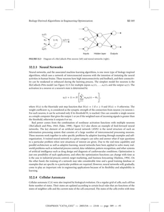
Best estimate = 0.046346
0 100 200 300 400 500 600
log[f(x)]
Best estimate = 0.23486
0 100 200 300 400 500 600
CHAPMAN: “C4754_C032” — 2005/5/6 — 23:44 — page 591 — #7
AQ: Please check
the change of
f (x) to f (x)
function and subsequently minimize the objective function f (x). However, there are many different ways
of defining a fitness function. For example, we can use the individual fitness assignment relative to the
whole population
F(xi ) =
f (xi )
N
i=1 f (xi )
,
where xi is the phenotypic value of individual i, and N is the population size. For the generalized
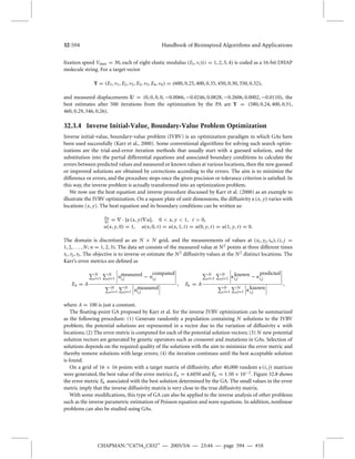
De Jong’s (1975) test function
f (x) =
n
i
=1
x2, |x| r , = 1, 2, . . . ,m,
where is a positive integer and r is the half-length of the domain. This function has a minimum of
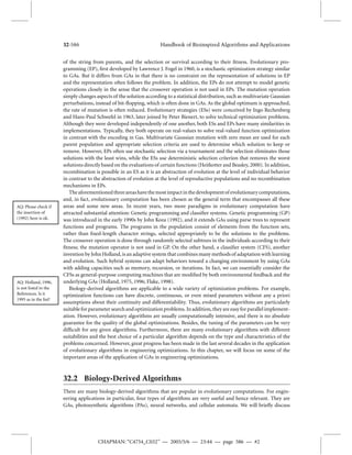
f (x) = 0 at x = 0. For the values of = 3, r = 256, and n = 40, the results of optimization of this test
function are shown in Figure 32.4 using GAs.
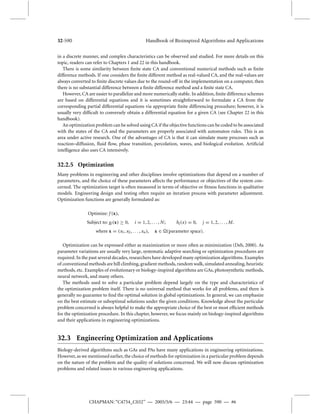
The function we just discussed is relatively simple in the sense that it is single-peaked. In reality, many
functions are multi-peaked and the optimization is thus multileveled. Keane (1995) studied the following
bumby function in a multi-peaked and multileveled optimization problem
f (x, y) =
sin2(x − y) sin2(x + y)
x2 + y2
, 0 x, y 10.
The optimization problem is to find (x, y) starting (5, 5) to maximize the function f (x, y) subject to:
x +y 15 and xy 3/4. In this problem, optimization is difficult because it is nearly symmetrical about
x = y, and while the peaks occur in pairs one is bigger than the other. In addition, the true maximum
is f (1.593, 0.471) = 0.365, which is defined by a constraint boundary. Figure 32.5 shows the surface
variation of the multi-peaked bumpy function.
Although the properties of this bumpy function make it difficult for most optimizers and algorithms,
GAs and other evolutionary algorithms performwell for this function and it has been widely used as a test
6
5
4
3
2
1
0
log[f(x)]
–1
–2
Generation (t)
6
5
4
3
2
1
0
–1
Generation (t)
FIGURE 32.4 Function optimization using GAs. Two runs will give slightly different results due to the stochastic
nature of GAs, but they produce better estimates: f (x) 0 as the generation increases.

8. 32-592 Handbook of Bioinspired Algorithms and Applications
0.6
0.4
0.2
0
0
5
10
0
5
y
x
10
f (x,y)
FIGURE 32.5 Surface of the multi-peaked bumpy function.
R
Th
Ts
R
L
FIGURE 32.6 Diagram of the pressure vessel.
function in GAs for comparative studies of various evolutionary algorithms or in multilevel optimization
environments (El-Beltagy and Keane, 1999).
32.3.2 Shape Design and Optimization
Most engineering design problems, especially in shape design, aim to reduce the cost, weight, and volume
and increase the performance and quality of the products. The optimization process starts with the
transformation of design specification and descriptions into optimization functions and constraints. The
structure and parameters of a product depend on the functionality and manufacturability, and thus
considerable effort has been put into the modeling of the design process and search technique to find
the optimal solution in the search space, which comprises the set of all designs with all allowable values
of design parameters (Renner and Ekart, 2003). Genetic algorithms have been applied in many areas of
engineering design such as conceptual design, shape optimization, data fitting, and robot path design.
A well-studied example is the design of a pressure vessel (Kannan and Kramer, 1994; Coello, 2000) using
different algorithms such as augmented Lagrangian multiplier and GAs. Figure 32.6 shows the diagram
of the parameter notations of the pressure vessel. The vessel is cylindrical and capped at both ends by
hemispherical heads with four design variables: thickness of the shell Ts, thickness of the head Th, inner
radius R, and the length of the cylindrical part L. The objective of the design is to minimize the total
cost including that of the material, forming, as well as welding. Using the notation given by Kannan and
CHAPMAN: “C4754_C032” — 2005/5/6 — 23:44 — page 592 — #8

9. Biology-Derived Algorithms in Engineering Optimization 32-593
Kramer, the optimization problem can be expressed as:
Minimize: f (x) = 0.6224x1x2x3 + 1.7781x2x2
3 + 3.1611x2
1 x4 + 19.84x2
1 x3.
x = (x1, x2, x3, x4)T = (Ts, Th, R, L)T,
Subject to: g1(x) = −x1 + 0.0193x3 0, g2(x) = −x2 + 0.00954x3 0,
g3(x) = − x2
3 x4 − 4 x3
3 /3 + 1296000 0, g4(x) = x4 − 240 0.
The values for x1, x2 should be considered as integer multiples of 0.0625. Using the same constraints as
given in Coello (2000), the variables are in the ranges: 1 x1, x2 99, 10.0000 x3. x4 100.0000
(with a four-decimal precision). By coding the GAs with a population of 44-bit strings for each indi-vidual
(4-bits for x1 · x2; 18-bits for x3 · x4), similar to that by Wu and Chow (1994), we can solve
the optimization problem for the pressure vessel. After several runs, the best solution obtained is
x = (1.125, 0.625, 58.2906, 43.6926) with f (x) = 7197.9912$, which is compared with the results
x = (1.125, 0.625, 28.291, 43.690) and f (x) = 7198.0428$ obtained by Kannan and Kramer (1994).
32.3.3 Finite Element Inverse Analysis
The usage and efficiency ofMurase’s PA described in Section 32.3.4 can be demonstrated in the application
of finite element inverse analysis. Finite element analysis (FEA) in structural engineering is forward
modeling as the aims are to calculate the displacements at various positions for given loading conditions
and material properties such as Young’s modulus (E) and Poisson’s ratio (
). This forward FEA is widely
used in engineering design and applications. Sometimes, inverse problems need to be solved. For a given
structure with known loading conditions andmeasured displacement, the objective is to find or invert the
material properties E and
, which may be required for testing new materials and design optimizations. It
is well known that inverse problems are usually very difficult, and this is especially true for finite element
inverse analysis.
To show how it works, we use a test example similar to that proposed byMurase (2000). A simple beam
system of 5 unit length × 10 unit length (see Figure 32.7) consists of five nodes and four elements whose
Young’s modulus and Poisson’s ratio may be different. Nodes 1 and 2 are fixed, and a unit vertical load is
applied at node 4 while the other nodes deform freely. Let us denote the displacement vector
U = (u1, v1, u2, v2, u3, v3, u4, v4, u5, v5)T,
where u1 = v1 = u2 = v2 = 0 (fixed). Measurements are made for other displacements. By using the PA
with the values of the CO2 affinity A = 10000, light intensity L = 104 to 5 × 104 lx, and maximum CO2
1
2
4
3
E4, n4
5
f =1
E1, n E3, n3 1
E2, n2
FIGURE 32.7 Beam system of finite element inverse analysis.
CHAPMAN: “C4754_C032” — 2005/5/6 — 23:44 — page 593 — #9

10. 32-594 Handbook of Bioinspired Algorithms and Applications
fixation speed Vmax = 30, each of eight elastic modulus (Ei ,
i )(i = 1, 2, 3, 4) is coded as a 16-bit DHAP
molecule string. For a target vector
Y = (E1,
1, E2,
2, E3,
3, E4,
4) = (600, 0.25, 400, 0.35, 450, 0.30, 350, 0.32),
and measured displacements U = (0, 0, 0, 0,−0.0066,−0.0246, 0.0828,−0.2606, 0.0002,−0.0110), the
best estimates after 500 iterations from the optimization by the PA are Y = (580, 0.24, 400, 0.31,
460, 0.29, 346, 0.26).
32.3.4 Inverse Initial-Value, Boundary-Value Problem Optimization
Inverse initial-value, boundary-value problem (IVBV) is an optimization paradigm in which GAs have
been used successfully (Karr et al., 2000). Some conventional algorithms for solving such search optim-izations
are the trial-and-error iteration methods that usually start with a guessed solution, and the
substitution into the partial differential equations and associated boundary conditions to calculate the
errors between predicted values andmeasured or known values at various locations, then the new guessed
or improved solutions are obtained by corrections according to the errors. The aim is to minimize the
difference or errors, and the procedure stops once the given precision or tolerance criterion is satisfied. In
this way, the inverse problem is actually transformed into an optimization problem.
We now use the heat equation and inverse procedure discussed by Karr et al. (2000) as an example to
illustrate the IVBV optimization. On a square plate of unit dimensions, the diffusivity (x, y) varies with
locations (x, y). The heat equation and its boundary conditions can be written as:

11. u

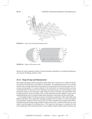
12. t =
· [(x, y)
u], 0 x, y 1, t 0,
u(x, y, 0) = 1, u(x, 0, t ) = u(x, 1, t ) = u(0, y, t ) = u(1, y, t ) = 0.
The domain is discretized as an N × N grid, and the measurements of values at (xi , yj , tn), (i, j =
1, 2, . . . ,N; n = 1, 2, 3). The data set consists of the measured value at N2 points at three different times
t1, t2, t3. The objective is to inverse or estimate the N2 diffusivity values at the N2 distinct locations. The
Karr’s error metrics are defined as
i=1N
j=1
i=1N
j=1
CHAPMAN: “C4754_C032” — 2005/5/6 — 23:44 — page 594 — #10
Eu = A
N
j=1
umeasured
i,j − u
computed
i,j
N
i=1N
umeasured
i,j
, E = A
N
j=1
known
i,j −
predicted
i,j
N
i=1N
known
i,j
,
where A = 100 is just a constant.
The floating-point GA proposed by Karr et al. for the inverse IVBV optimization can be summarized
as the following procedure: (1) Generate randomly a population containing N solutions to the IVBV
problem; the potential solutions are represented in a vector due to the variation of diffusivity with
locations; (2) The errormetric is computed for each of the potential solution vectors; (3) N new potential
solution vectors are generated by genetic operators such as crossover and mutations in GAs. Selection of
solutions depends on the required quality of the solutions with the aim to minimize the error metric and
thereby remove solutions with large errors; (4) the iteration continues until the best acceptable solution
is found.
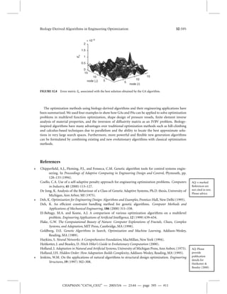
On a grid of 16 × 16 points with a target matrix of diffusivity, after 40,000 random (i, j) matrices
were generated, the best value of the error metrics Eu = 4.6050 and E = 1.50×10−2. Figure 32.8 shows
the error metric E associated with the best solution determined by the GA. The small values in the error
metric imply that the inverse diffusivity matrix is very close to the true diffusivity matrix.
With some modifications, this type of GA can also be applied to the inverse analysis of other problems
such as the inverse parametric estimation of Poisson equation and wave equations. In addition, nonlinear
problems can also be studied using GAs.