derivatives. maximum and minimum value..

1. Copyright © Cengage Learning. All rights reserved.
14 Partial Derivatives

2. Copyright © Cengage Learning. All rights reserved.
14.7 Maximum and Minimum Values

3. 3
3
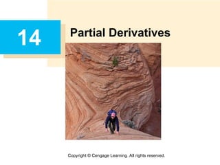
Maximum and Minimum Values
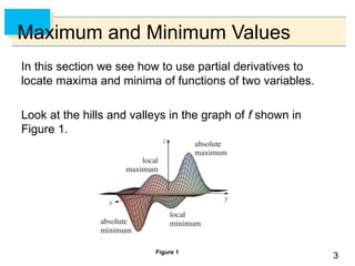
In this section we see how to use partial derivatives to
locate maxima and minima of functions of two variables.
Look at the hills and valleys in the graph of f shown in
Figure 1.
Figure 1

4. 4
4
Maximum and Minimum Values
There are two points (a, b) where f has a local maximum,
that is, where f(a, b) is larger than nearby values of f(x, y).
The larger of these two values is the absolute maximum.
Likewise, f has two local minima, where f(a, b) is smaller
than nearby values.
The smaller of these two values is the absolute minimum.

5. 5
5
Maximum and Minimum Values
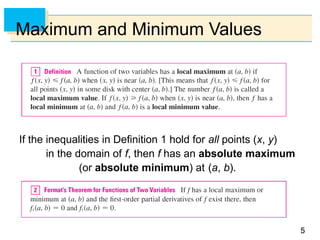
If the inequalities in Definition 1 hold for all points (x, y)
in the domain of f, then f has an absolute maximum
(or absolute minimum) at (a, b).

6. 6
6
Maximum and Minimum Values
A point (a, b) is called a critical point (or stationary point)
of f if fx(a, b) = 0 and fy(a, b) = 0, or if one of these partial
derivatives does not exist.
Theorem 2 says that if f has a local maximum or minimum
at (a, b), then (a, b) is a critical point of f.
However, as in single-variable calculus, not all critical
points give rise to maxima or minima.
At a critical point, a function could have a local maximum or
a local minimum or neither.

7. 7
7
Example 1
Let f(x, y) = x2
+ y2
– 2x – 6y + 14.
Then
fx(x, y) = 2x – 2 fy(x, y) = 2y – 6
These partial derivatives are equal to 0 when x = 1 and
y = 3, so the only critical point is (1, 3).
By completing the square, we find that
f(x, y) = 4 + (x – 1)2
+ (y – 3)2

8. 8
8
Example 1
Since (x – 1)2
 0 and (y – 3)2
 0, we have f(x, y)  4 for
all values of x and y.
Therefore f(1, 3) = 4 is a local minimum, and in fact it is the
absolute minimum of f.
This can be confirmed geometrically from the graph of f,
which is the elliptic paraboloid with vertex (1, 3, 4) shown in
Figure 2.
cont’d
Figure 2
z = x2
+ y2
– 2x – 6y + 14

9. 9
9
Maximum and Minimum Values
The following test, is analogous to the Second Derivative
Test for functions of one variable.
In case (c) the point (a, b) is called a saddle point of f and
the graph of f crosses its tangent plane at (a, b).

10. 10
10
Absolute Maximum and
Minimum Values

11. 11
11
Absolute Maximum and Minimum Values
For a function f of one variable, the Extreme Value
Theorem says that if f is continuous on a closed interval [a,
b], then f has an absolute minimum value and an absolute
maximum value.
According to the Closed Interval Method, we found these
by evaluating f not only at the critical numbers but also at
the endpoints a and b.
There is a similar situation for functions of two variables.

12. 12
12
Absolute Maximum and Minimum Values
Just as a closed interval contains its endpoints, a closed
set in is one that contains all its boundary points.
[A boundary point of D is a point (a, b) such that every disk
with center (a, b) contains points in D and also points not in
D.]
For instance, the disk
D = {(x, y)| x2
+ y2
 1}
which consists of all points on and inside the circle
x2
+ y2
= 1, is a closed set because it contains all of its
boundary points (which are the points on the circle
x2
+ y2
= 1).

13. 13
13
Absolute Maximum and Minimum Values
But if even one point on the boundary curve were omitted,
the set would not be closed. (See Figure 11.)
Figure 11

14. 14
14
Absolute Maximum and Minimum Values
A bounded set in is one that is contained within some
disk.
In other words, it is finite in extent.
Then, in terms of closed and bounded sets, we can state
the following counterpart of the Extreme Value Theorem in
two dimensions.

15. 15
15
Absolute Maximum and Minimum Values
To find the extreme values guaranteed by Theorem 8, we
note that, by Theorem 2, if f has an extreme value at
(x1, y1), then (x1, y1) is either a critical point of f or a
boundary point of D.
Thus we have the following extension of the Closed Interval
Method.

16. 16
16
Example 7
Find the absolute maximum and minimum values of the
function f(x, y) = x2
– 2xy + 2y on the rectangle
D = {(x, y)|0  x  3, 0  y  2}.
Solution:
Since f is a polynomial, it is continuous on the closed,
bounded rectangle D, so Theorem 8 tells us there is both
an absolute maximum and an absolute minimum.
According to step 1 in , we first find the critical points.

17. 17
17
Example 7 – Solution
These occur when
fx = 2x – 2y = 0 fy = –2x + 2 = 0
so the only critical point is (1, 1), and the value of f there is
f(1, 1) = 1.
In step 2 we look at the values of f on the boundary of D,
which consists of the four line segments L1, L2, L3, L4
shown in Figure 12.
cont’d
Figure 12

18. 18
18
Example 7 – Solution
On L1 we have y = 0 and
f(x, 0) = x2
0  x  3
This is an increasing function of x, so its minimum value is
f(0, 0) = 0 and its maximum value is f(3, 0) = 9.
On L2 we have x = 3 and
f(3, y) = 9 – 4y 0  y  2
This is a decreasing function of y, so its maximum value is
f(3, 0) = 9 and its minimum value is f(3, 2) = 1.
cont’d

19. 19
19
Example 7 – Solution
On L3 we have y = 2 and
f(x, 2) = x2
– 4x + 4 0  x  3
Simply by observing that f(x, 2) = (x – 2)2
, we see
that the minimum value of this function is f(2, 2) = 0 and the
maximum value is f(0, 2) = 4.
cont’d

20. 20
20
Example 7 – Solution
Finally, on L4 we have x = 0 and
f(0, y) = 2y 0  y  2
with maximum value f(0, 2) = 4 and minimum value
f(0, 0) = 0.
Thus, on the boundary, the minimum value of f is 0 and the
maximum is 9.
cont’d

21. 21
21
Example 7 – Solution
In step 3 we compare these values with the value
f(1, 1) = 1 at the critical point and conclude that the
absolute maximum value of f on D is f(3, 0) = 9 and the
absolute minimum value is f(0, 0) = f(2, 2) = 0.
Figure 13 shows the graph of f.
Figure 13
f(x, y) = x2
– 2xy + 2y
cont’d