Downloaded 160 times


![Example
The Schema H = [0 1 ∗ 1 *] generates the following individuals
0 1 * 1 *
0 1 0 1 0
0 1 0 1 1
0 1 1 1 0
0 1 1 1 1
Not all schemas say the same
Schema [ 1 ∗ ∗ ∗ ∗ ∗ ∗] has less information than [ 0 1 ∗ ∗ 1 1 0].
It is more!!!
[ 1 ∗ ∗ ∗ ∗ ∗ 0] span the entire length of an individual, but
[ 1 ∗ 1 ∗ ∗ ∗ ∗] does not.
6 / 37](https://image.slidesharecdn.com/07-150406005645-conversion-gate01/75/07-2-Holland-s-Genetic-Algorithms-Schema-Theorem-12-2048.jpg)
![Example
The Schema H = [0 1 ∗ 1 *] generates the following individuals
0 1 * 1 *
0 1 0 1 0
0 1 0 1 1
0 1 1 1 0
0 1 1 1 1
Not all schemas say the same
Schema [ 1 ∗ ∗ ∗ ∗ ∗ ∗] has less information than [ 0 1 ∗ ∗ 1 1 0].
It is more!!!
[ 1 ∗ ∗ ∗ ∗ ∗ 0] span the entire length of an individual, but
[ 1 ∗ 1 ∗ ∗ ∗ ∗] does not.
6 / 37](https://image.slidesharecdn.com/07-150406005645-conversion-gate01/75/07-2-Holland-s-Genetic-Algorithms-Schema-Theorem-13-2048.jpg)
![Example
The Schema H = [0 1 ∗ 1 *] generates the following individuals
0 1 * 1 *
0 1 0 1 0
0 1 0 1 1
0 1 1 1 0
0 1 1 1 1
Not all schemas say the same
Schema [ 1 ∗ ∗ ∗ ∗ ∗ ∗] has less information than [ 0 1 ∗ ∗ 1 1 0].
It is more!!!
[ 1 ∗ ∗ ∗ ∗ ∗ 0] span the entire length of an individual, but
[ 1 ∗ 1 ∗ ∗ ∗ ∗] does not.
6 / 37](https://image.slidesharecdn.com/07-150406005645-conversion-gate01/75/07-2-Holland-s-Genetic-Algorithms-Schema-Theorem-14-2048.jpg)


![Then
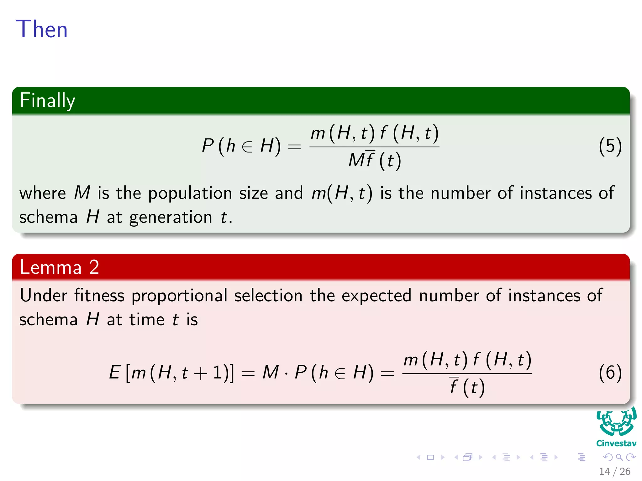
Finally
P (h ∈ H) =
m (H, t) f (H, t)
Mf (t)
(5)
where M is the population size and m(H, t) is the number of instances of
schema H at generation t.
Lemma 2
Under fitness proportional selection the expected number of instances of
schema H at time t is
E [m (H, t + 1)] = M · P (h ∈ H) =
m (H, t) f (H, t)
f (t)
(6)
18 / 37](https://image.slidesharecdn.com/07-150406005645-conversion-gate01/75/07-2-Holland-s-Genetic-Algorithms-Schema-Theorem-46-2048.jpg)
![Then
Finally
P (h ∈ H) =
m (H, t) f (H, t)
Mf (t)
(5)
where M is the population size and m(H, t) is the number of instances of
schema H at generation t.
Lemma 2
Under fitness proportional selection the expected number of instances of
schema H at time t is
E [m (H, t + 1)] = M · P (h ∈ H) =
m (H, t) f (H, t)
f (t)
(6)
18 / 37](https://image.slidesharecdn.com/07-150406005645-conversion-gate01/75/07-2-Holland-s-Genetic-Algorithms-Schema-Theorem-47-2048.jpg)
![Why?
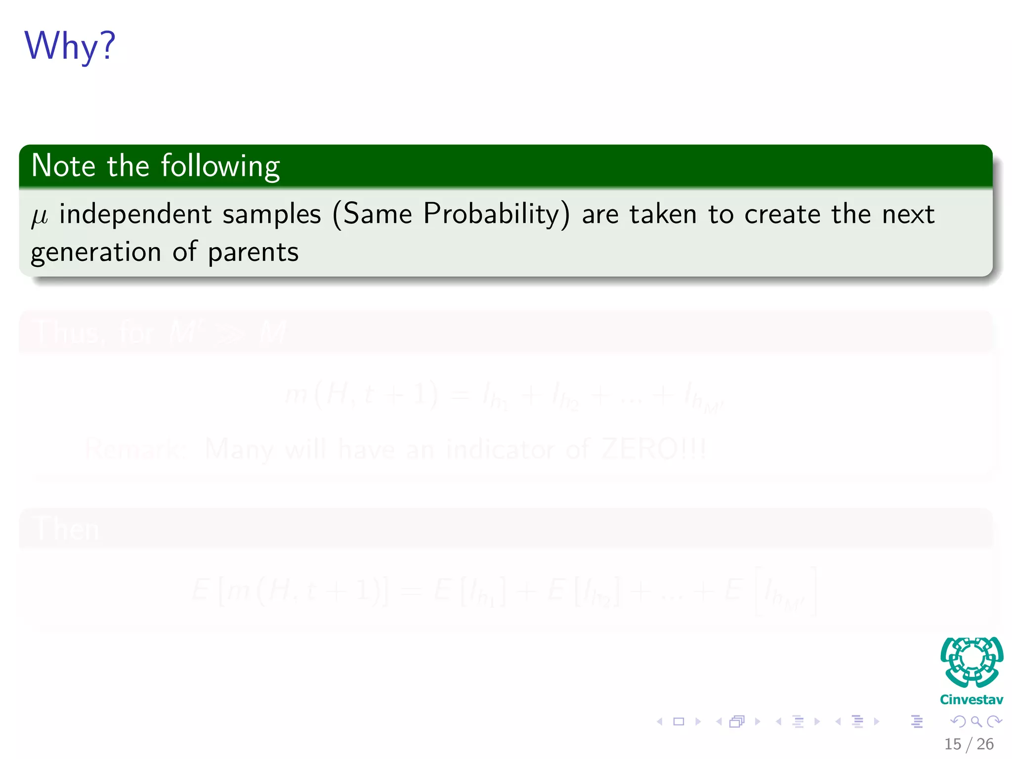
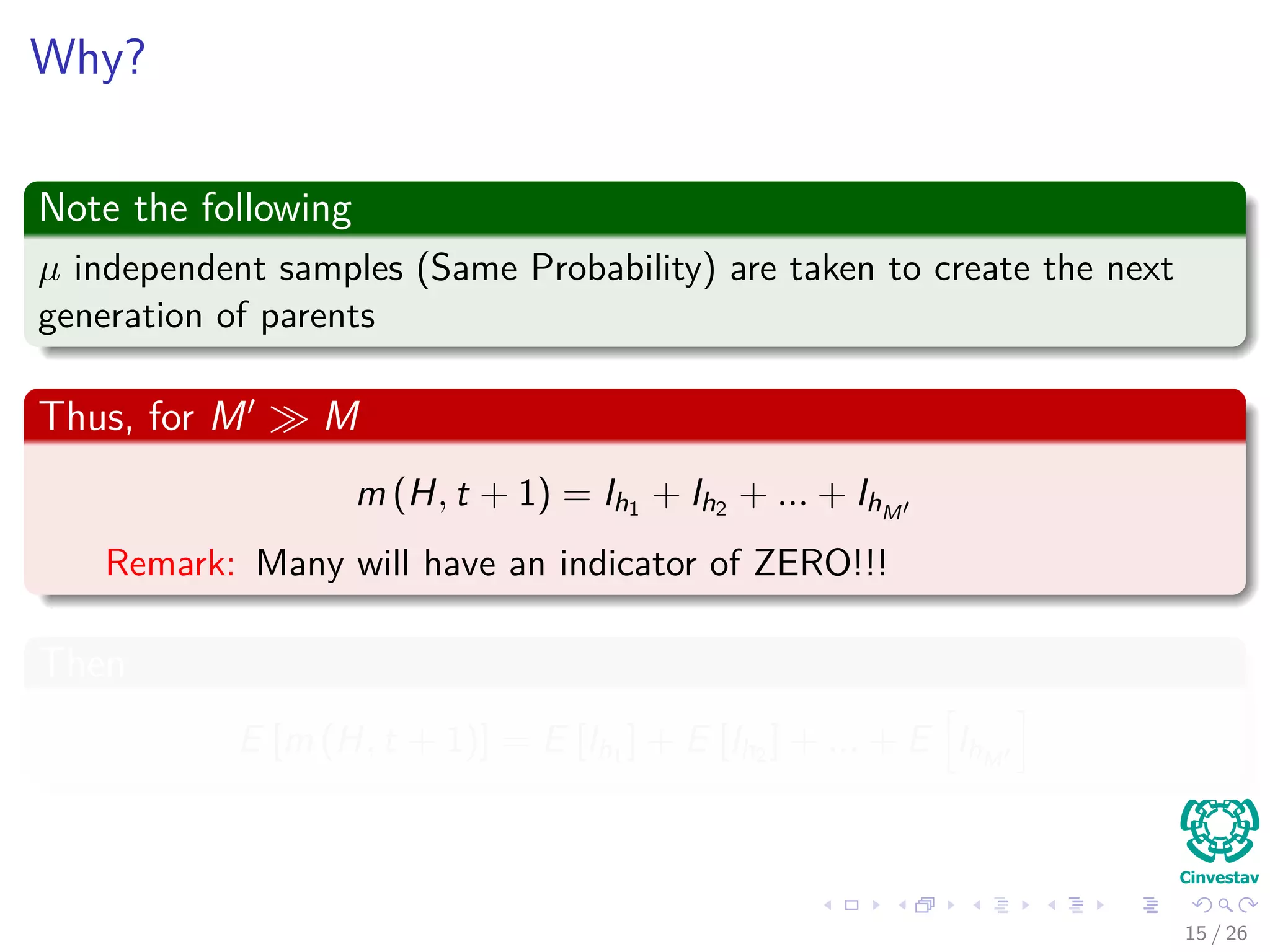
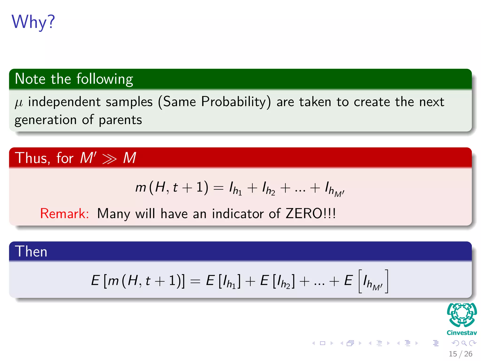
Note the following
M independent samples (Same Probability) are taken to create the next
generation of parents
Thus
m (H, t + 1) = Ih1 + Ih2 + ... + IhM
Remark: The indicator random variable of ONE for these samples!!!
Then
E [m (H, t + 1)] = E [Ih1 ] + E [Ih2 ] + ... + E [IhM
]
19 / 37](https://image.slidesharecdn.com/07-150406005645-conversion-gate01/75/07-2-Holland-s-Genetic-Algorithms-Schema-Theorem-48-2048.jpg)
![Why?
Note the following
M independent samples (Same Probability) are taken to create the next
generation of parents
Thus
m (H, t + 1) = Ih1 + Ih2 + ... + IhM
Remark: The indicator random variable of ONE for these samples!!!
Then
E [m (H, t + 1)] = E [Ih1 ] + E [Ih2 ] + ... + E [IhM
]
19 / 37](https://image.slidesharecdn.com/07-150406005645-conversion-gate01/75/07-2-Holland-s-Genetic-Algorithms-Schema-Theorem-49-2048.jpg)
![Why?
Note the following
M independent samples (Same Probability) are taken to create the next
generation of parents
Thus
m (H, t + 1) = Ih1 + Ih2 + ... + IhM
Remark: The indicator random variable of ONE for these samples!!!
Then
E [m (H, t + 1)] = E [Ih1 ] + E [Ih2 ] + ... + E [IhM
]
19 / 37](https://image.slidesharecdn.com/07-150406005645-conversion-gate01/75/07-2-Holland-s-Genetic-Algorithms-Schema-Theorem-50-2048.jpg)
![Finally
But, M samples are taken to create the next generation of parents
E [m (H, t + 1)] = P (h1 ∈ H) + P (h2 ∈ H) + ... + P (hM ∈ H)
Remember the Lemma 5.1 in Cormen’s Book
Finally, because P (h1 ∈ H) = P (h2 ∈ H) = ... = P (hM ∈ H)
E [m (H, t + 1)] = M × P (h ∈ H)
QED!!!
20 / 37](https://image.slidesharecdn.com/07-150406005645-conversion-gate01/75/07-2-Holland-s-Genetic-Algorithms-Schema-Theorem-51-2048.jpg)
![Finally
But, M samples are taken to create the next generation of parents
E [m (H, t + 1)] = P (h1 ∈ H) + P (h2 ∈ H) + ... + P (hM ∈ H)
Remember the Lemma 5.1 in Cormen’s Book
Finally, because P (h1 ∈ H) = P (h2 ∈ H) = ... = P (hM ∈ H)
E [m (H, t + 1)] = M × P (h ∈ H)
QED!!!
20 / 37](https://image.slidesharecdn.com/07-150406005645-conversion-gate01/75/07-2-Holland-s-Genetic-Algorithms-Schema-Theorem-52-2048.jpg)
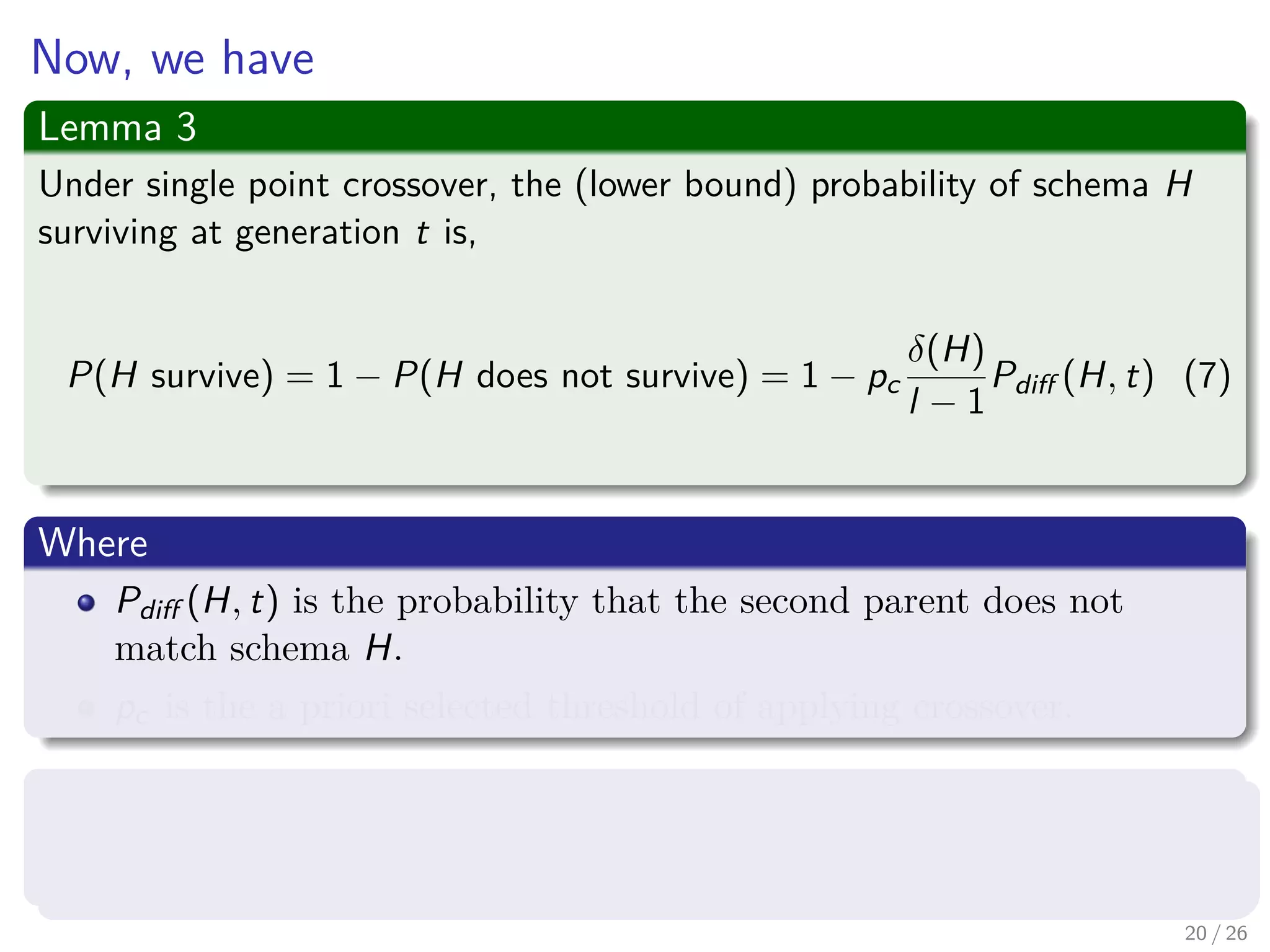
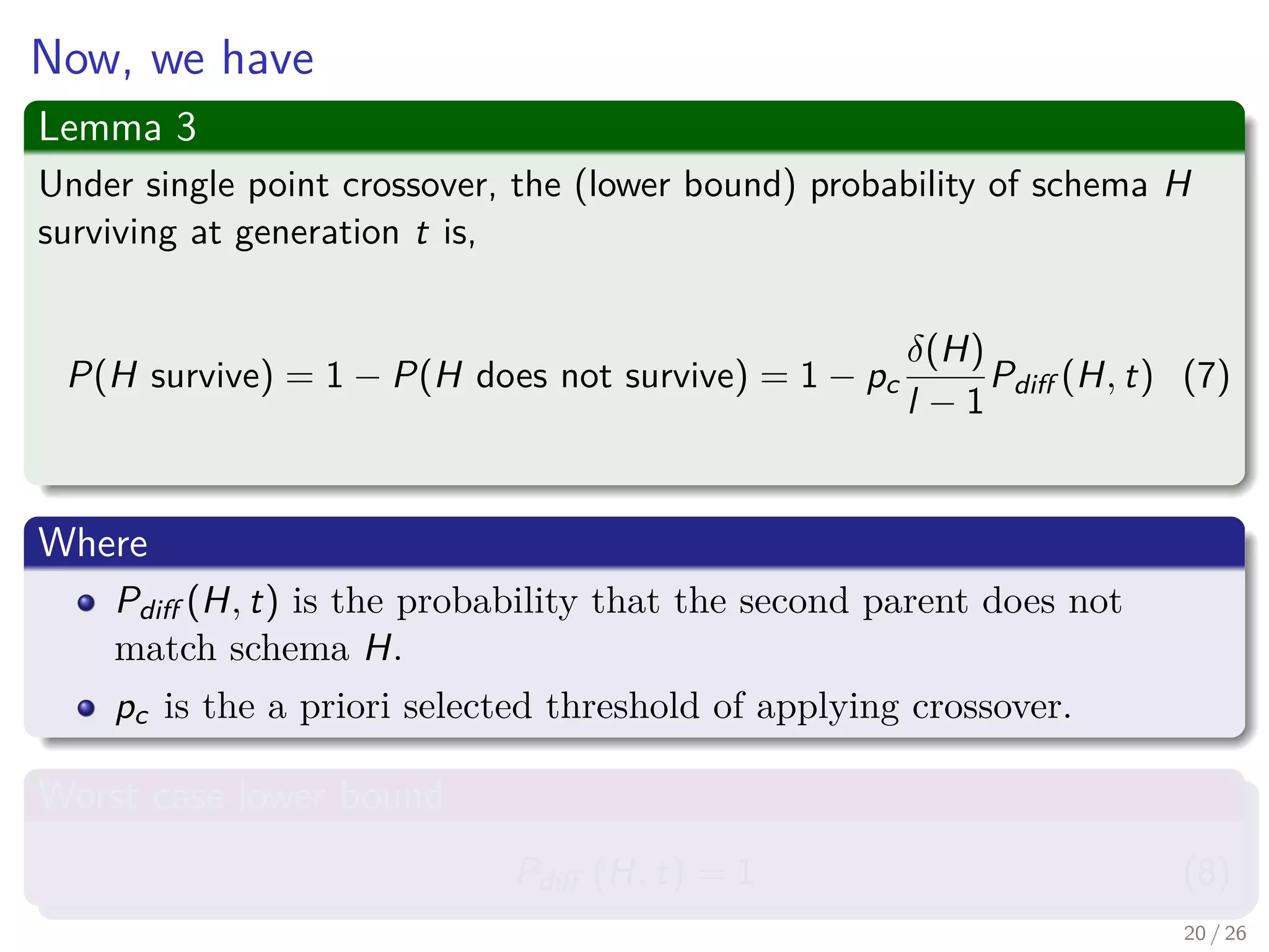
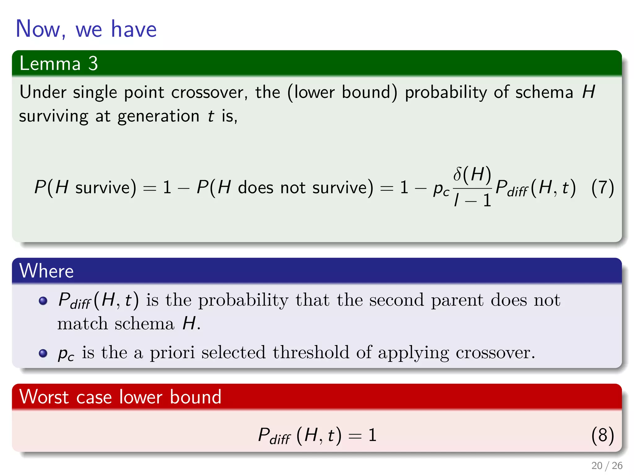

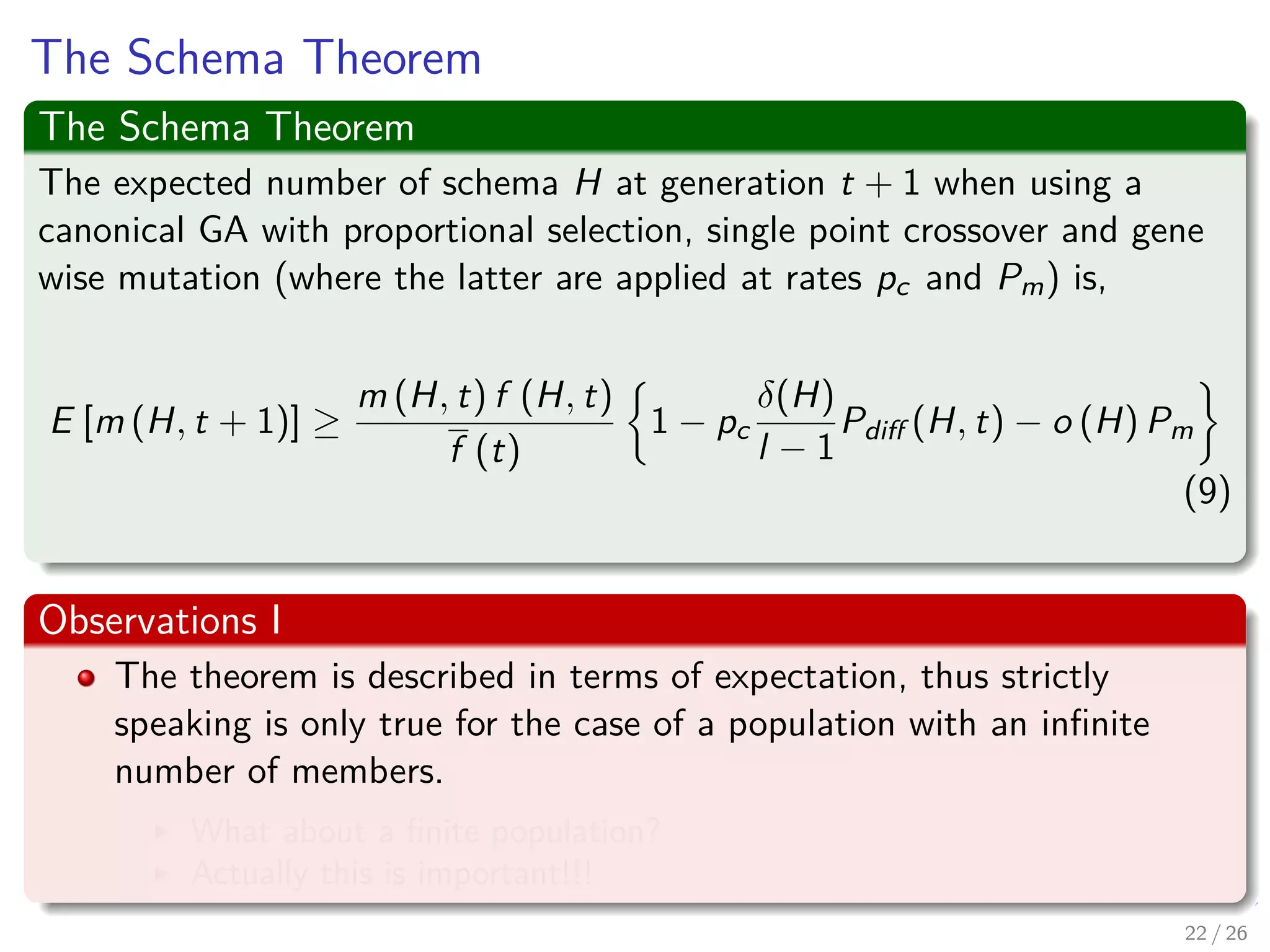

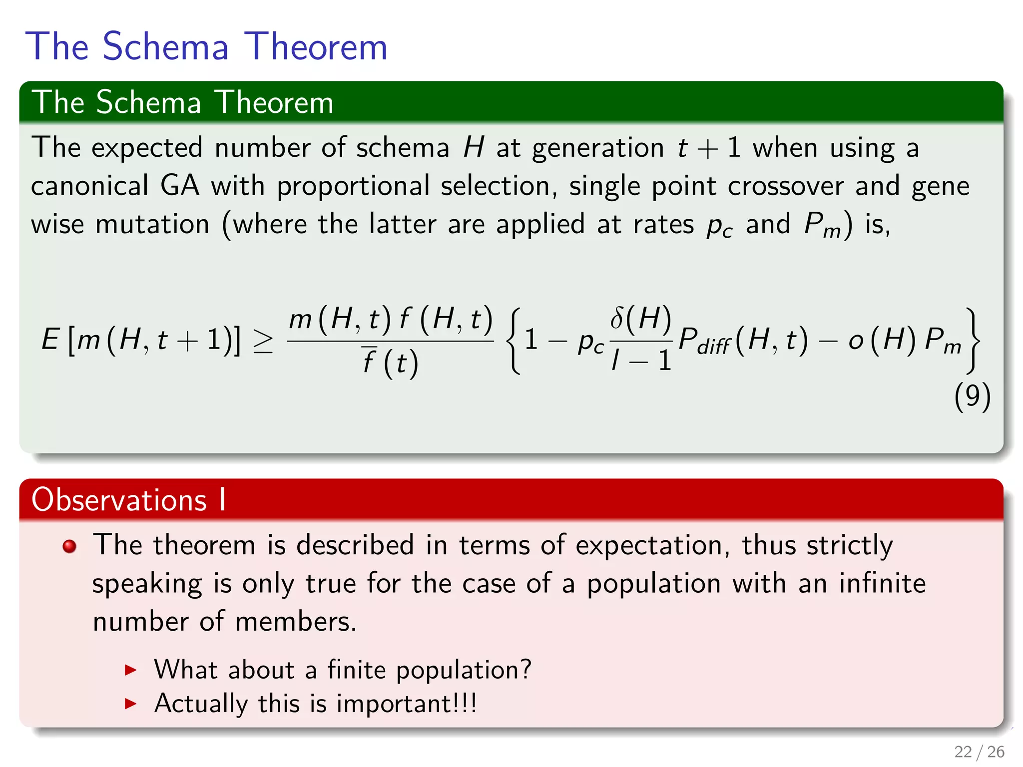


![The Schema Theorem
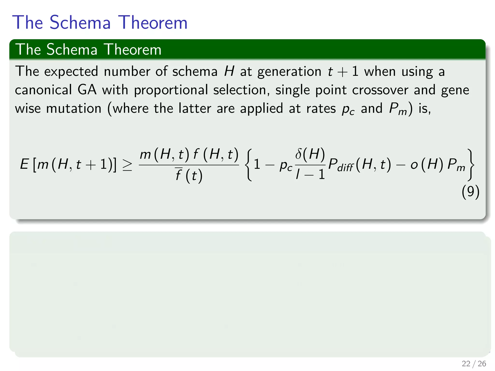
The Schema Theorem
The expected number of schema H at generation t + 1 when using a
canonical GA with proportional selection, single point crossover and gene
wise mutation (where the latter are applied at rates pc and Pm) is,
E [m (H, t + 1)] ≥
m (H, t) f (H, t)
f (t)
1 − pc
δ(H)
l − 1
Pdiff (H, t) − o (H) Pm
(8)
28 / 37](https://image.slidesharecdn.com/07-150406005645-conversion-gate01/75/07-2-Holland-s-Genetic-Algorithms-Schema-Theorem-69-2048.jpg)
![Proof
We use the following quantities
Pcrossover (H survive) = 1 − pc
δ(H)
l−1 Pdiff (H, t) ≤ 1
Pno−disruption (H, mutation) = 1 − o (H) Pm ≤ 1
Then, we have that
E [m (H, t + 1)] =M × P (h ∈ H)
=M
m (H, t) f (H, t)
Mf (t)
=
m (H, t) f (H, t)
f (t)
≥
m (H, t) f (H, t)
f (t)
× 1 − pc
δ(H)
l − 1
Pdiff (H, t) × [1 − o (H) Pm]
29 / 37](https://image.slidesharecdn.com/07-150406005645-conversion-gate01/75/07-2-Holland-s-Genetic-Algorithms-Schema-Theorem-70-2048.jpg)
![Proof
We use the following quantities
Pcrossover (H survive) = 1 − pc
δ(H)
l−1 Pdiff (H, t) ≤ 1
Pno−disruption (H, mutation) = 1 − o (H) Pm ≤ 1
Then, we have that
E [m (H, t + 1)] =M × P (h ∈ H)
=M
m (H, t) f (H, t)
Mf (t)
=
m (H, t) f (H, t)
f (t)
≥
m (H, t) f (H, t)
f (t)
× 1 − pc
δ(H)
l − 1
Pdiff (H, t) × [1 − o (H) Pm]
29 / 37](https://image.slidesharecdn.com/07-150406005645-conversion-gate01/75/07-2-Holland-s-Genetic-Algorithms-Schema-Theorem-71-2048.jpg)
![Proof
We use the following quantities
Pcrossover (H survive) = 1 − pc
δ(H)
l−1 Pdiff (H, t) ≤ 1
Pno−disruption (H, mutation) = 1 − o (H) Pm ≤ 1
Then, we have that
E [m (H, t + 1)] =M × P (h ∈ H)
=M
m (H, t) f (H, t)
Mf (t)
=
m (H, t) f (H, t)
f (t)
≥
m (H, t) f (H, t)
f (t)
× 1 − pc
δ(H)
l − 1
Pdiff (H, t) × [1 − o (H) Pm]
29 / 37](https://image.slidesharecdn.com/07-150406005645-conversion-gate01/75/07-2-Holland-s-Genetic-Algorithms-Schema-Theorem-72-2048.jpg)
![Thus
We have the following
E [m (H, t + 1)] ≥
m (H, t) f (H, t)
f (t)
1 − pc
δ(H)
l − 1
Pdiff (H, t) − o (H) Pm + ...
pc
δ(H)
l − 1
Pdiff (H, t)o (H) Pm
≥
m (H, t) f (H, t)
f (t)
1 − pc
δ(H)
l − 1
Pdiff (H, t) − o (H) Pm
The las inequality is possible because pc
δ(H)
l−1 Pdiff (H, t)o (H) Pm ≥ 0
30 / 37](https://image.slidesharecdn.com/07-150406005645-conversion-gate01/75/07-2-Holland-s-Genetic-Algorithms-Schema-Theorem-73-2048.jpg)


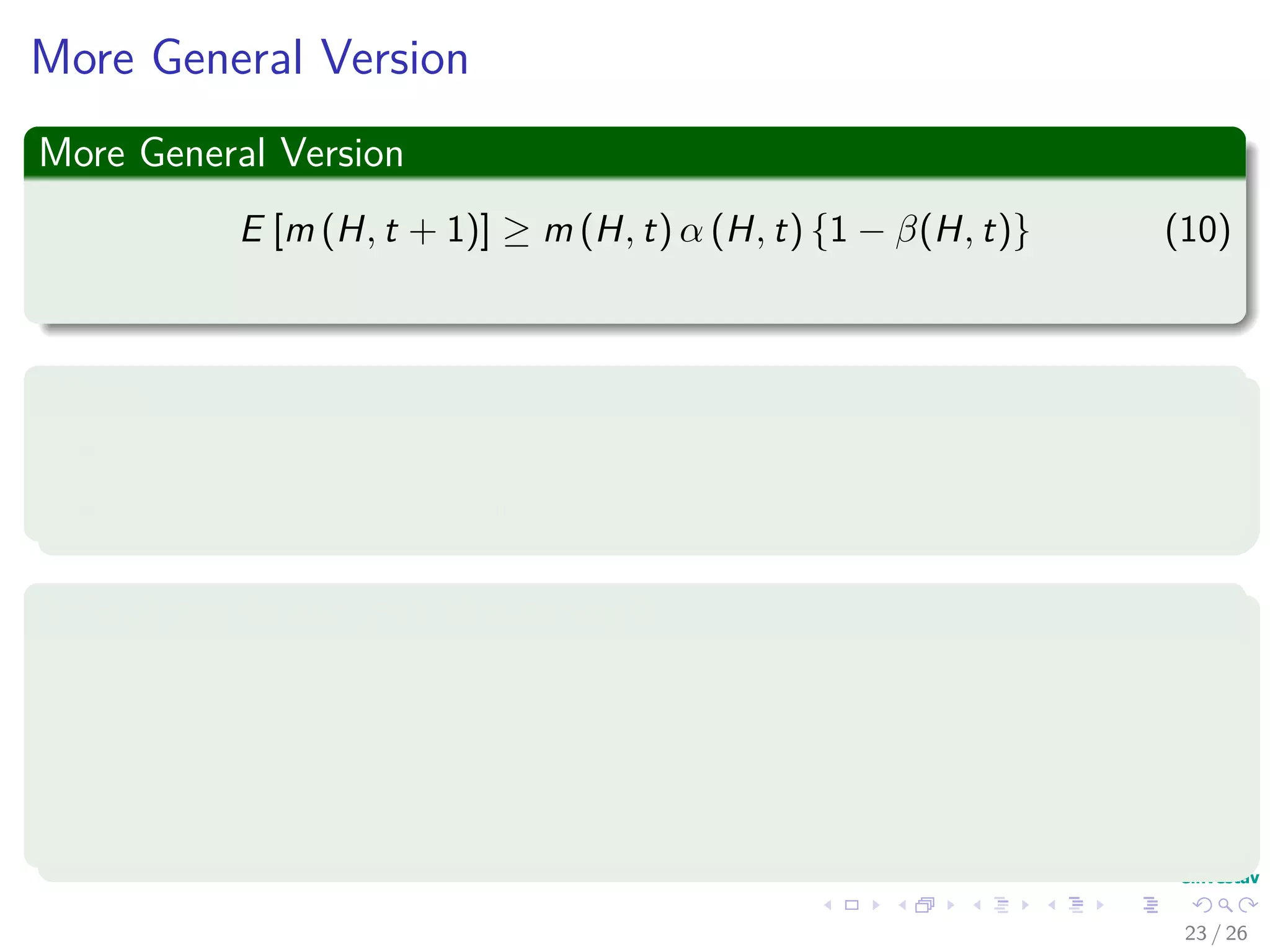
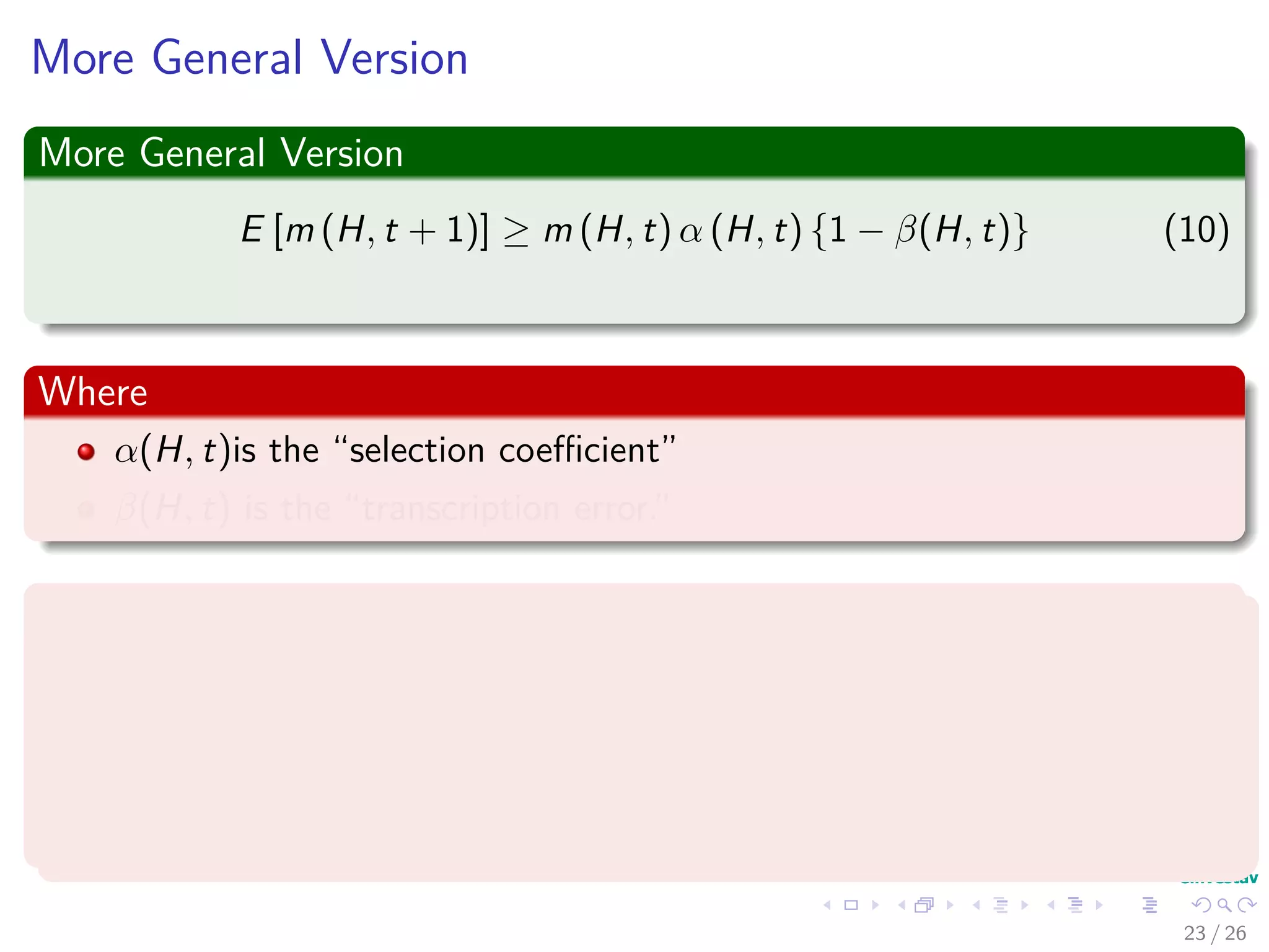
![More General Version
More General Version
E [m (H, t + 1)] ≥ m (H, t) α (H, t) {1 − β(H, t)} (9)
Where
α(H, t)is the “selection coefficient”
β(H, t) is the “transcription error.”
This allows to say that H survives if
α(H, t) ≥ 1 − β (H, t) or
m (H, t) f (H, t)
f (t)
≥ 1 − pc
δ(H)
l − 1
Pdiff (H, t) − o (H) Pm
33 / 37](https://image.slidesharecdn.com/07-150406005645-conversion-gate01/75/07-2-Holland-s-Genetic-Algorithms-Schema-Theorem-78-2048.jpg)
![More General Version
More General Version
E [m (H, t + 1)] ≥ m (H, t) α (H, t) {1 − β(H, t)} (9)
Where
α(H, t)is the “selection coefficient”
β(H, t) is the “transcription error.”
This allows to say that H survives if
α(H, t) ≥ 1 − β (H, t) or
m (H, t) f (H, t)
f (t)
≥ 1 − pc
δ(H)
l − 1
Pdiff (H, t) − o (H) Pm
33 / 37](https://image.slidesharecdn.com/07-150406005645-conversion-gate01/75/07-2-Holland-s-Genetic-Algorithms-Schema-Theorem-79-2048.jpg)
![More General Version
More General Version
E [m (H, t + 1)] ≥ m (H, t) α (H, t) {1 − β(H, t)} (9)
Where
α(H, t)is the “selection coefficient”
β(H, t) is the “transcription error.”
This allows to say that H survives if
α(H, t) ≥ 1 − β (H, t) or
m (H, t) f (H, t)
f (t)
≥ 1 − pc
δ(H)
l − 1
Pdiff (H, t) − o (H) Pm
33 / 37](https://image.slidesharecdn.com/07-150406005645-conversion-gate01/75/07-2-Holland-s-Genetic-Algorithms-Schema-Theorem-80-2048.jpg)
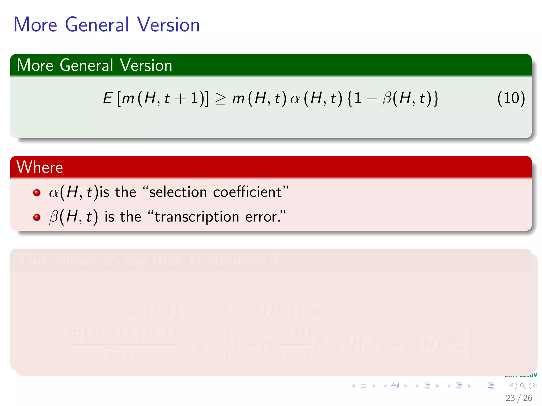
![More General Version
More General Version
E [m (H, t + 1)] ≥ m (H, t) α (H, t) {1 − β(H, t)} (9)
Where
α(H, t)is the “selection coefficient”
β(H, t) is the “transcription error.”
This allows to say that H survives if
α(H, t) ≥ 1 − β (H, t) or
m (H, t) f (H, t)
f (t)
≥ 1 − pc
δ(H)
l − 1
Pdiff (H, t) − o (H) Pm
33 / 37](https://image.slidesharecdn.com/07-150406005645-conversion-gate01/75/07-2-Holland-s-Genetic-Algorithms-Schema-Theorem-81-2048.jpg)


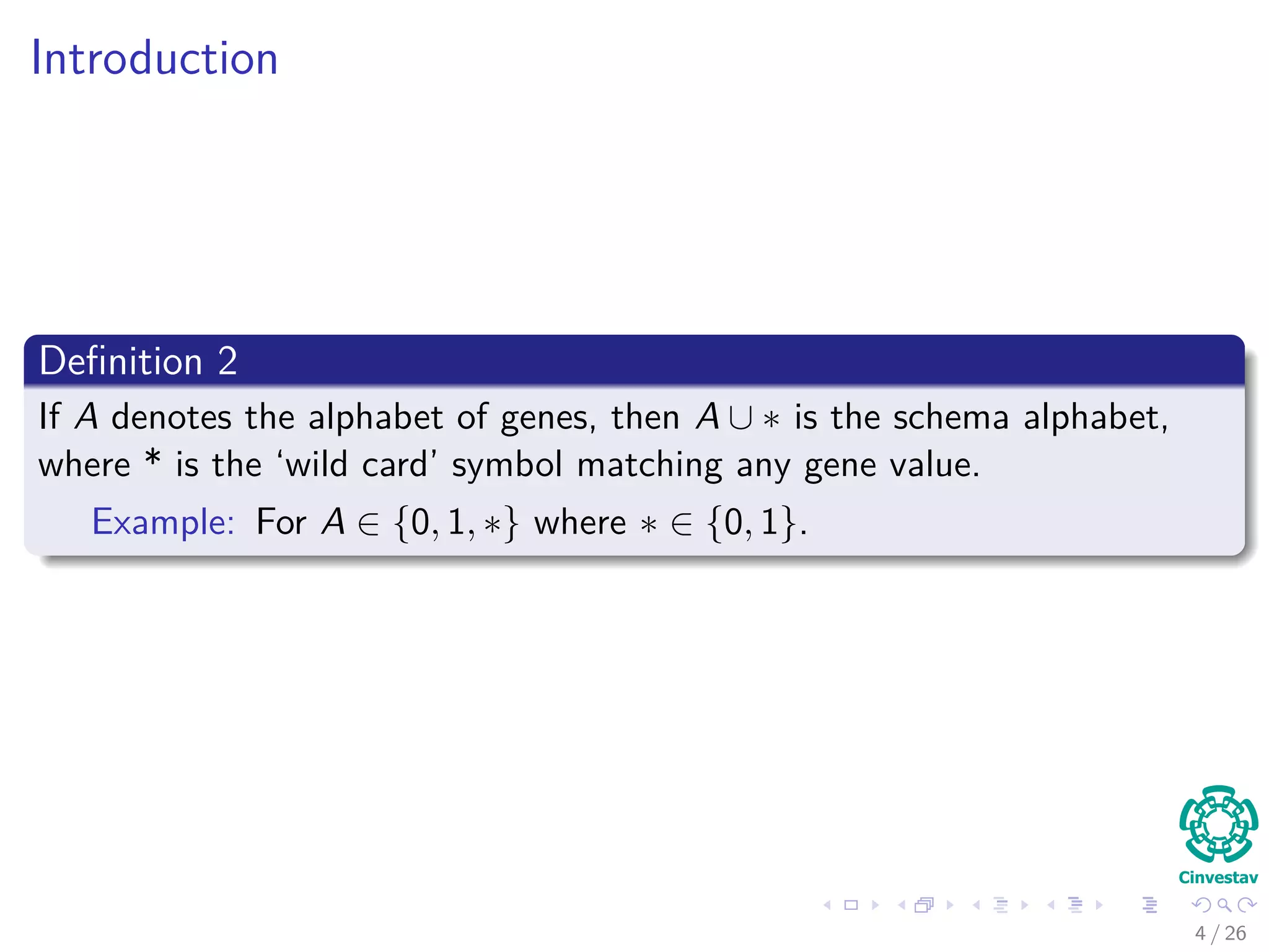
The document discusses the concept of schemas in genetic algorithms (GAs), defining schemas as templates that identify subsets of similar strings within a fixed-length binary alphabet. It elaborates on the properties of schemas, including their order and defining length, and explores the probabilities of schemas surviving various genetic operations such as mutation and crossover. Additionally, the document critiques the schema theorem and presents cases to illustrate the impact of mutations on the survival of these schemas.
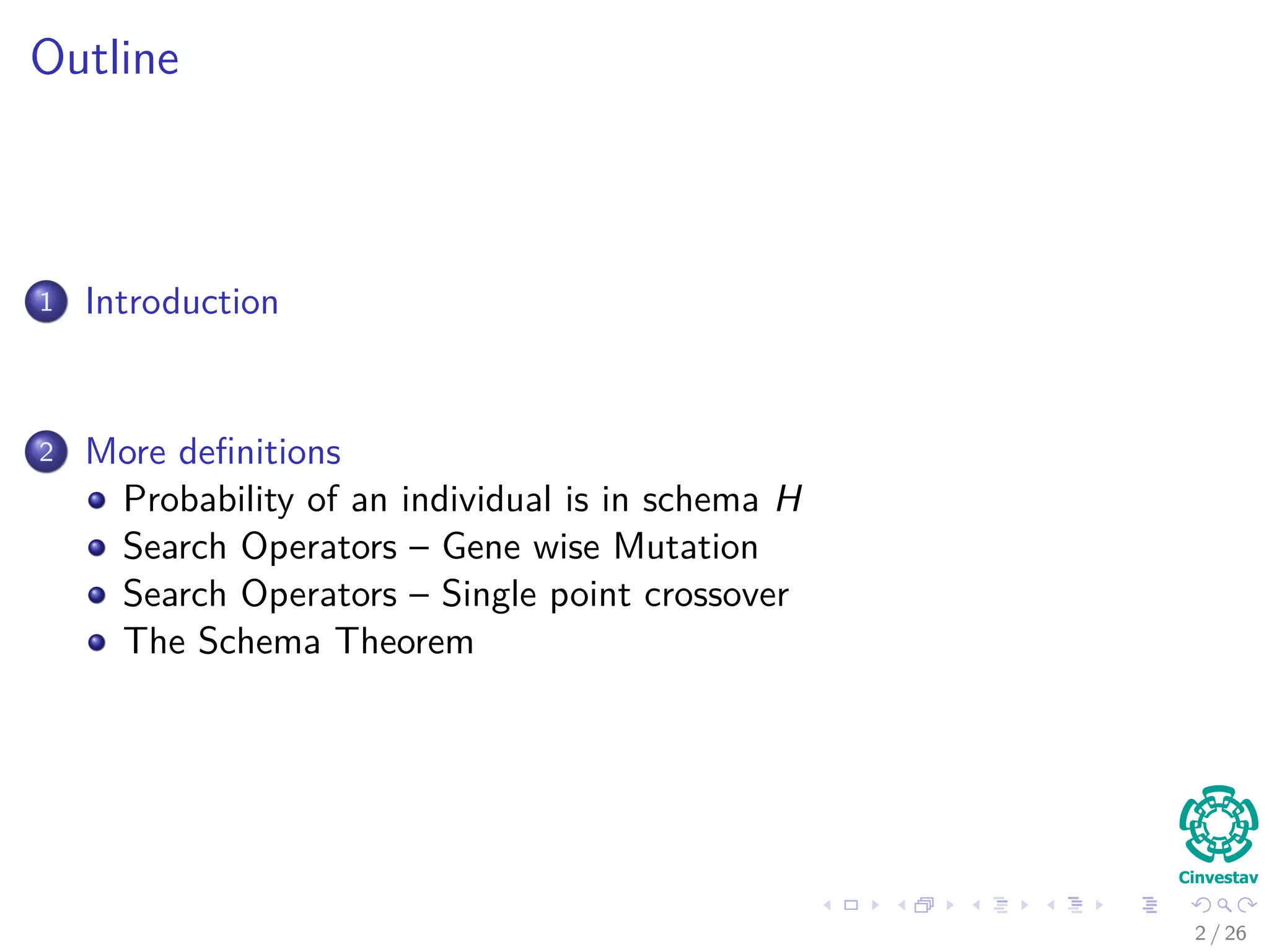
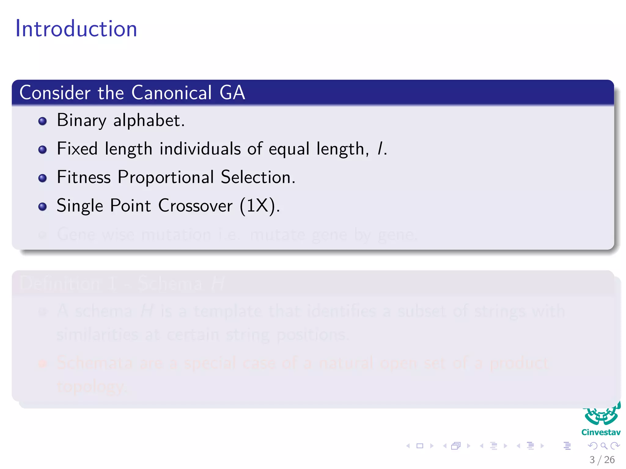
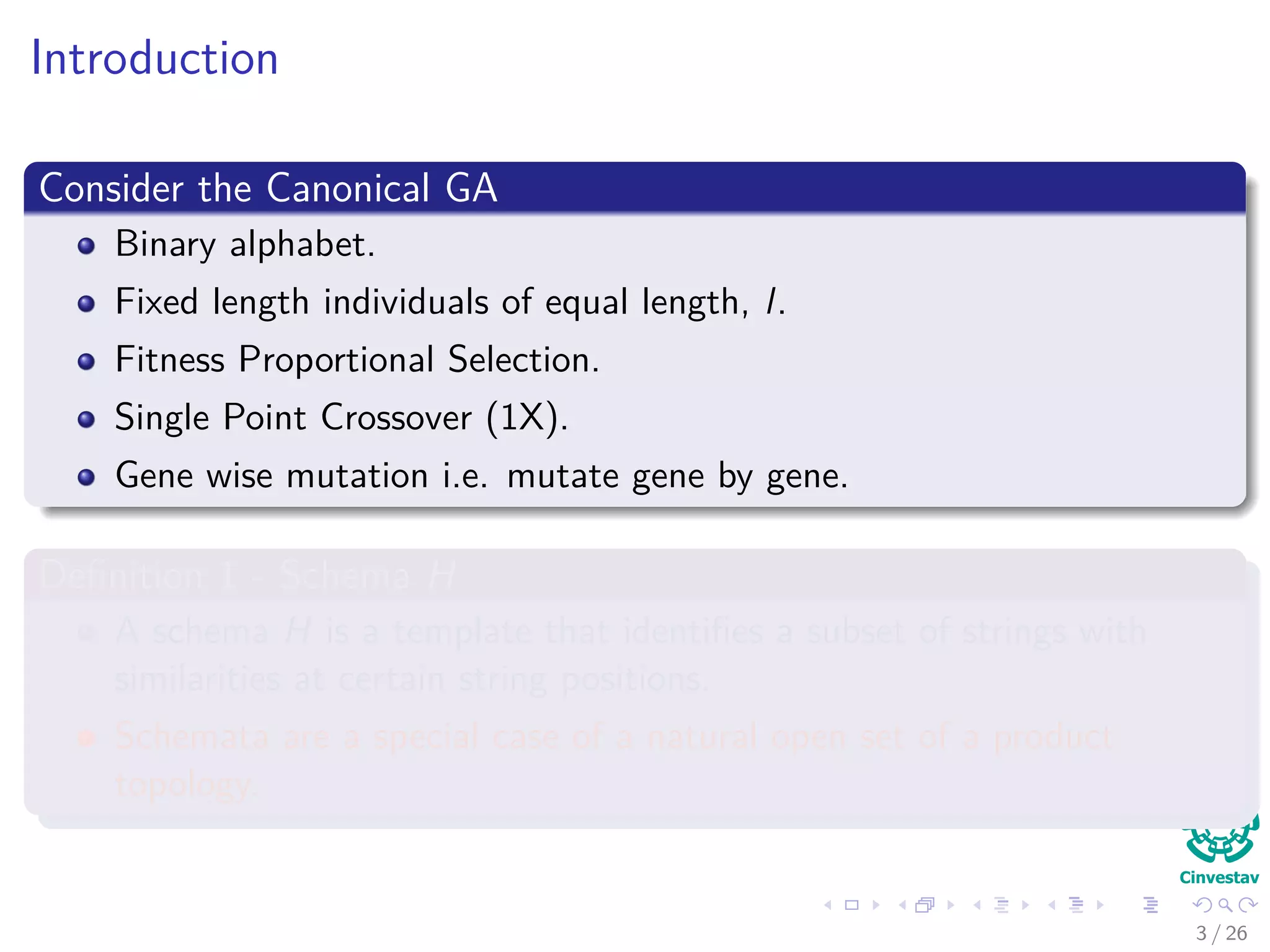
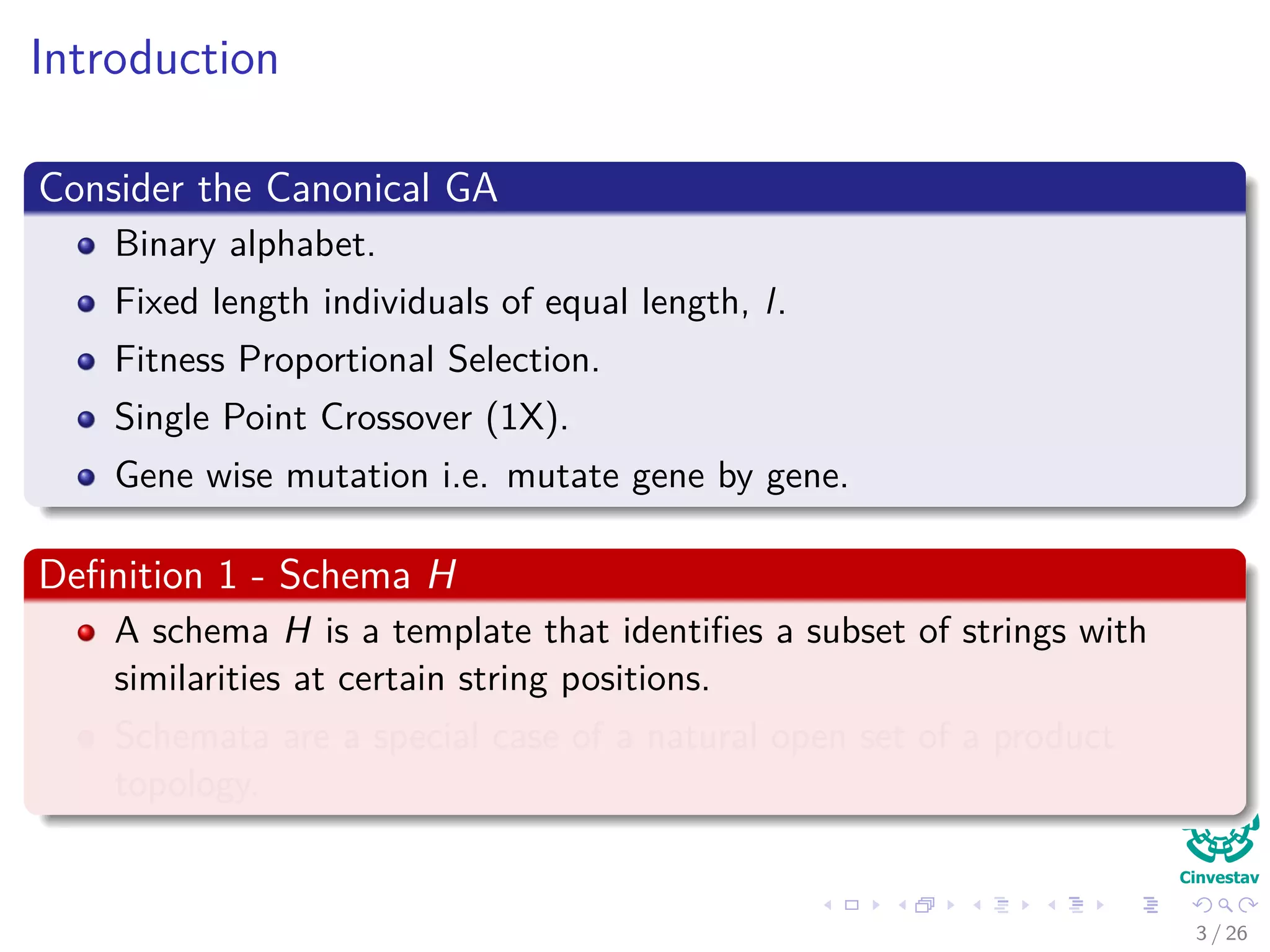
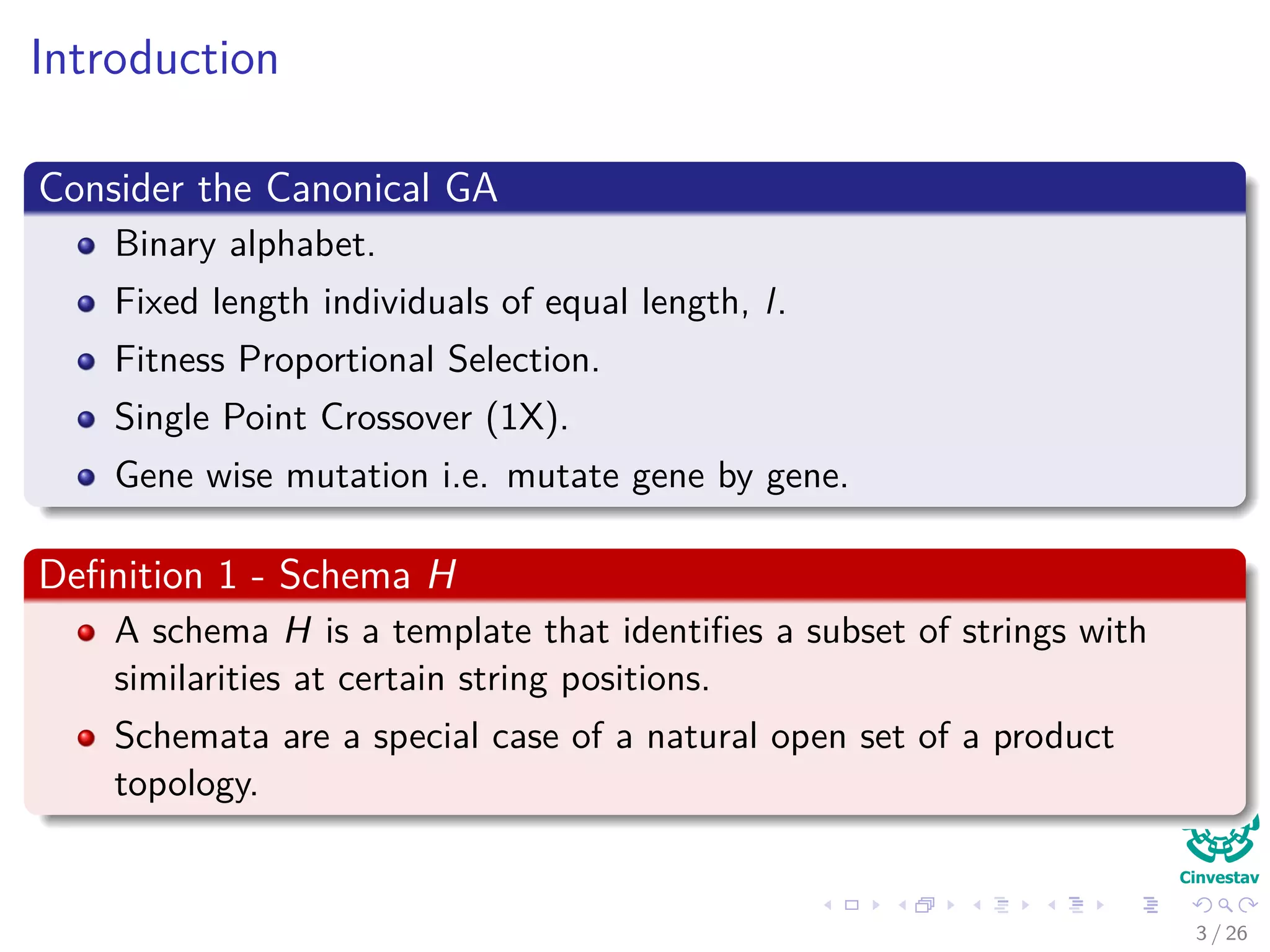
Overview of the presentation and definition of schema in Genetic Algorithms.
Detailed explanations of schema definitions and examples showcasing their generations.
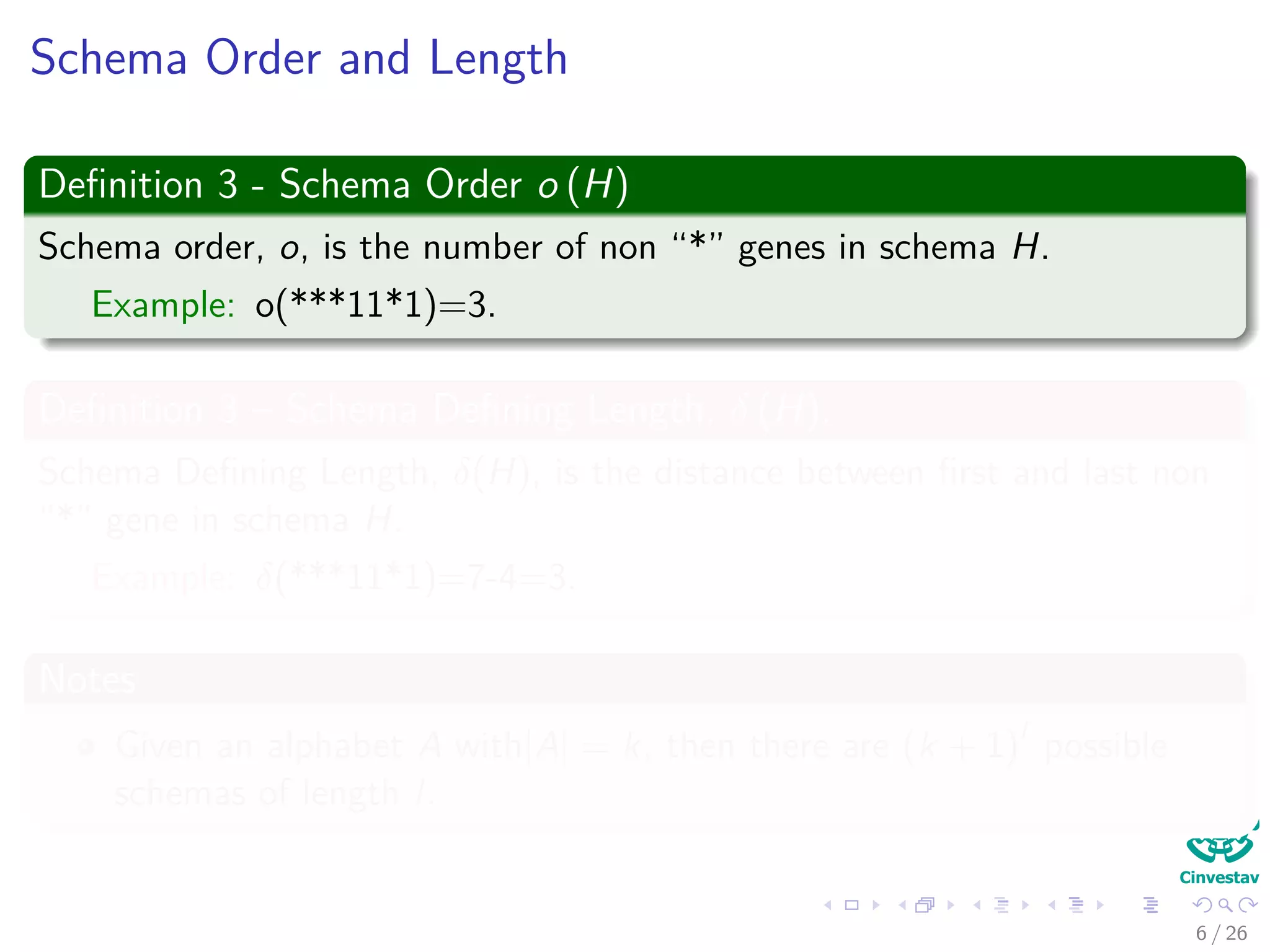
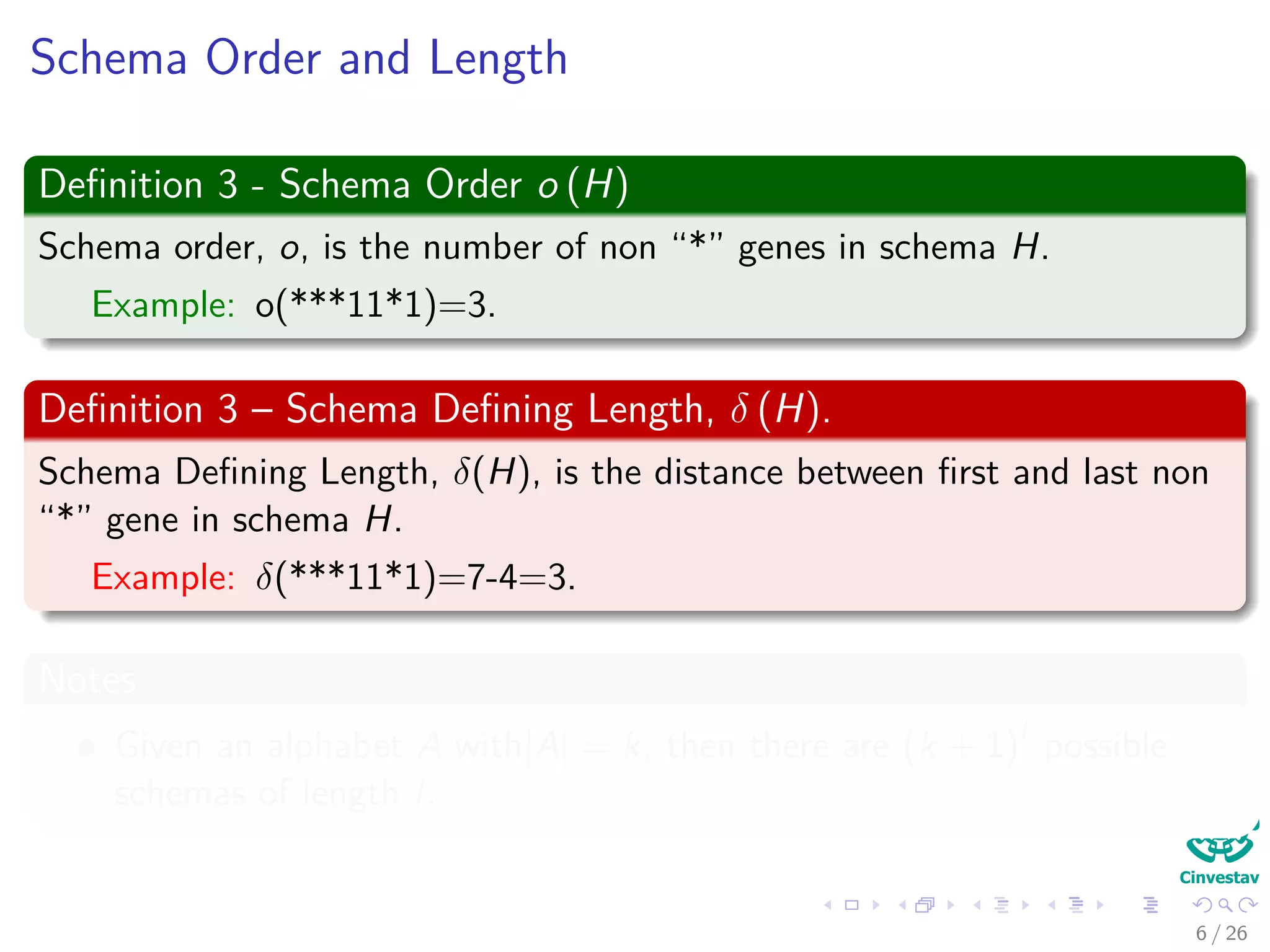
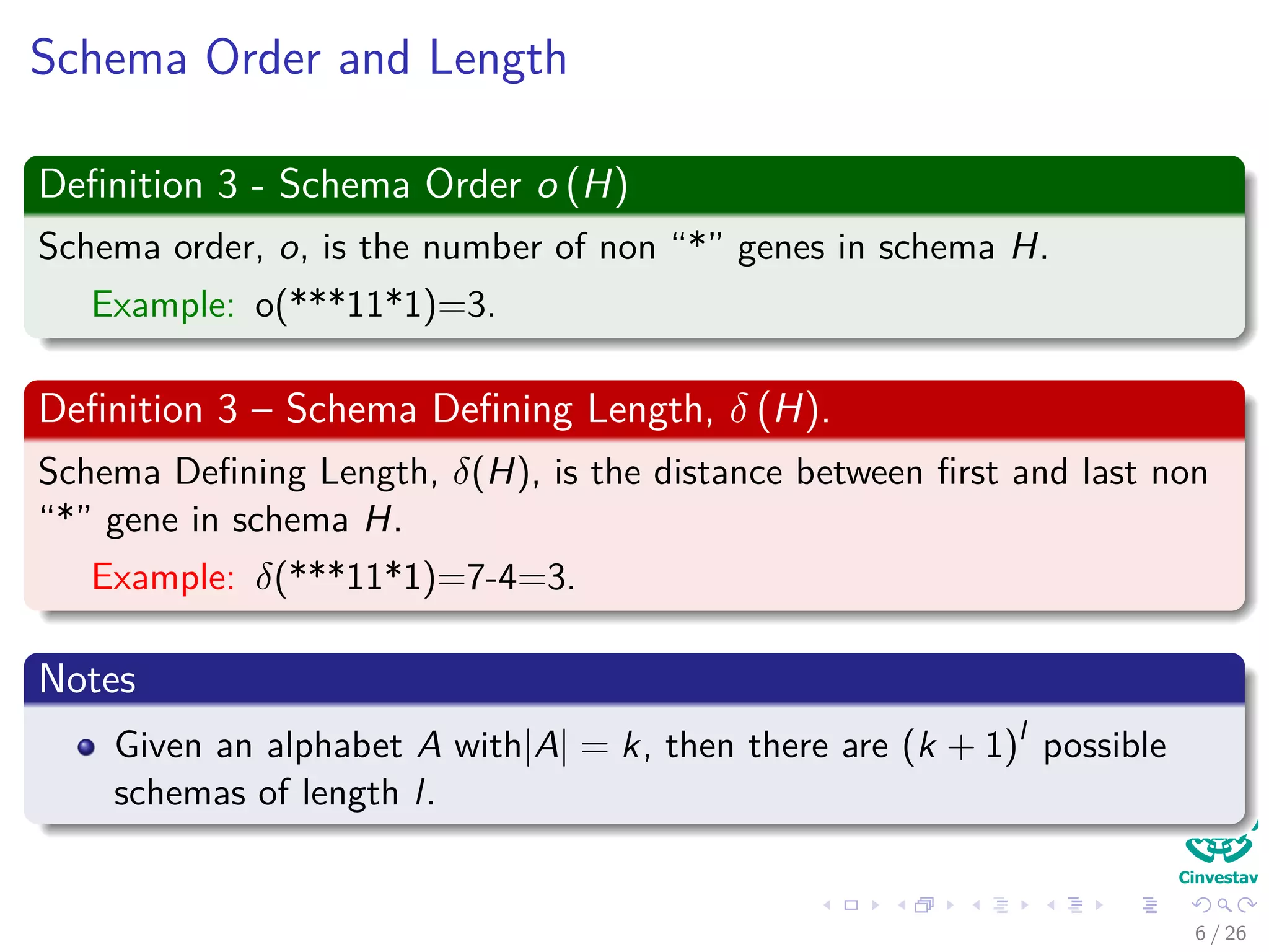
Introduction of schema order and defining length, along with related notes and notations.
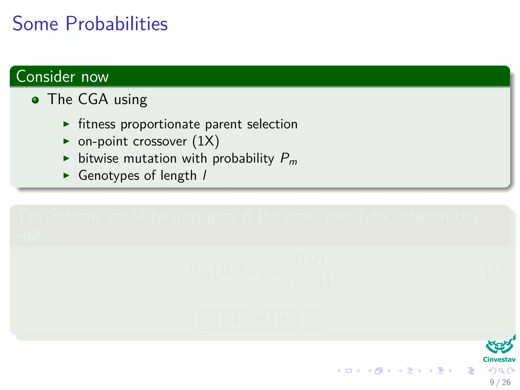
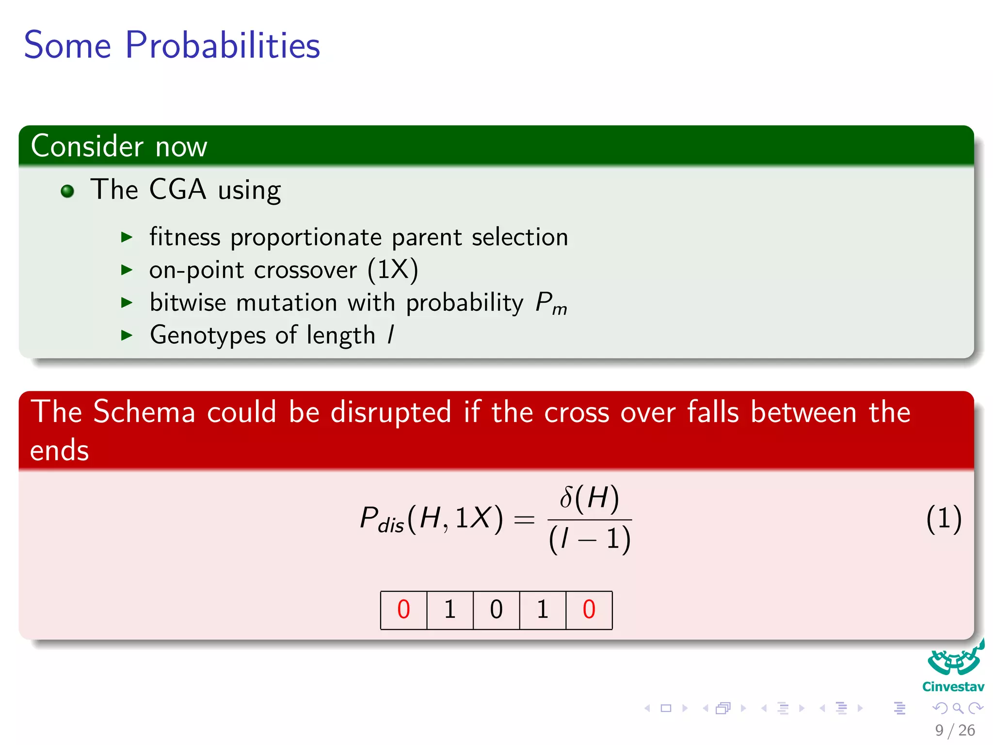
Probabilities related to the survival of schemas under mutations and crossover operations.
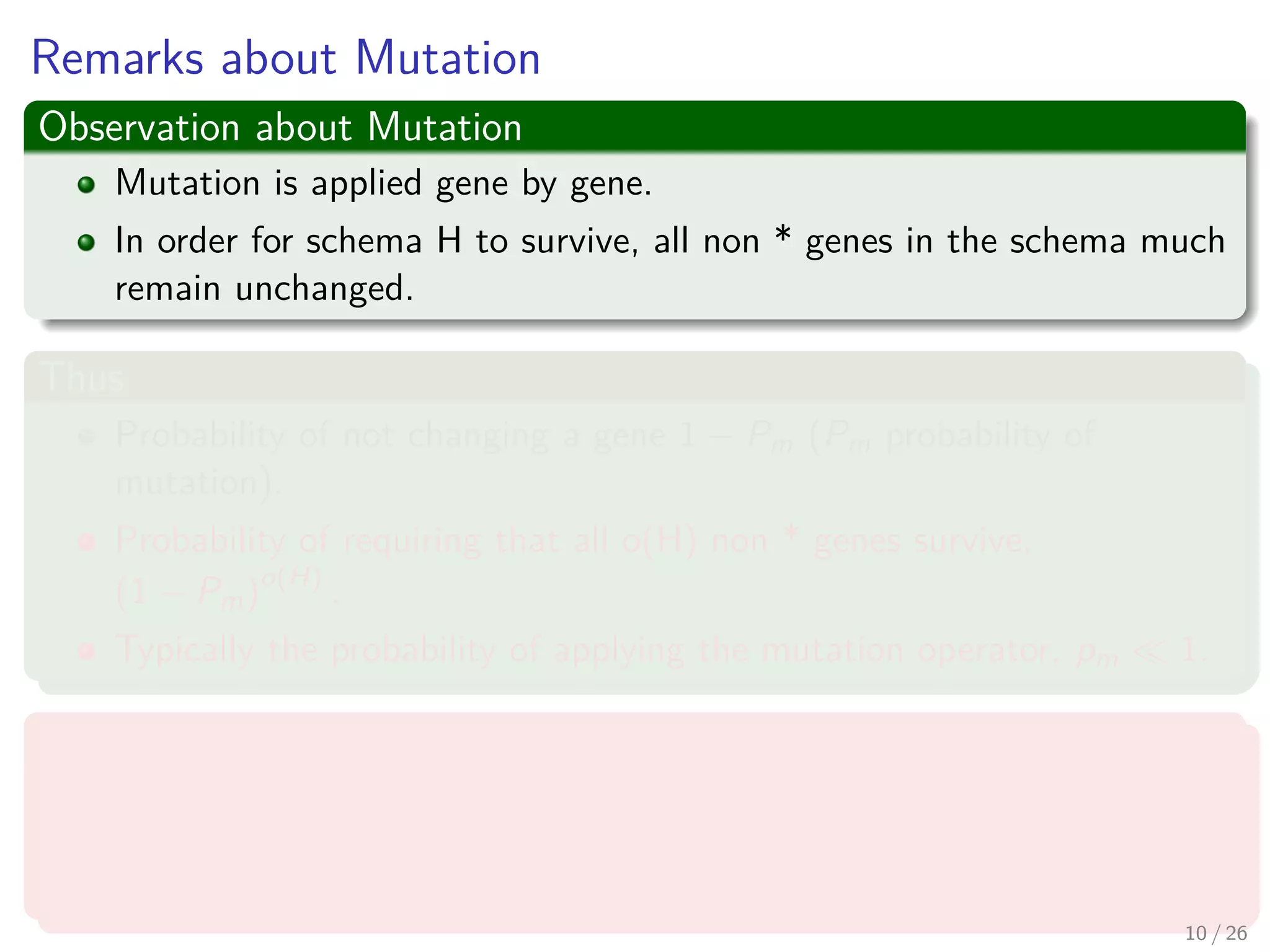
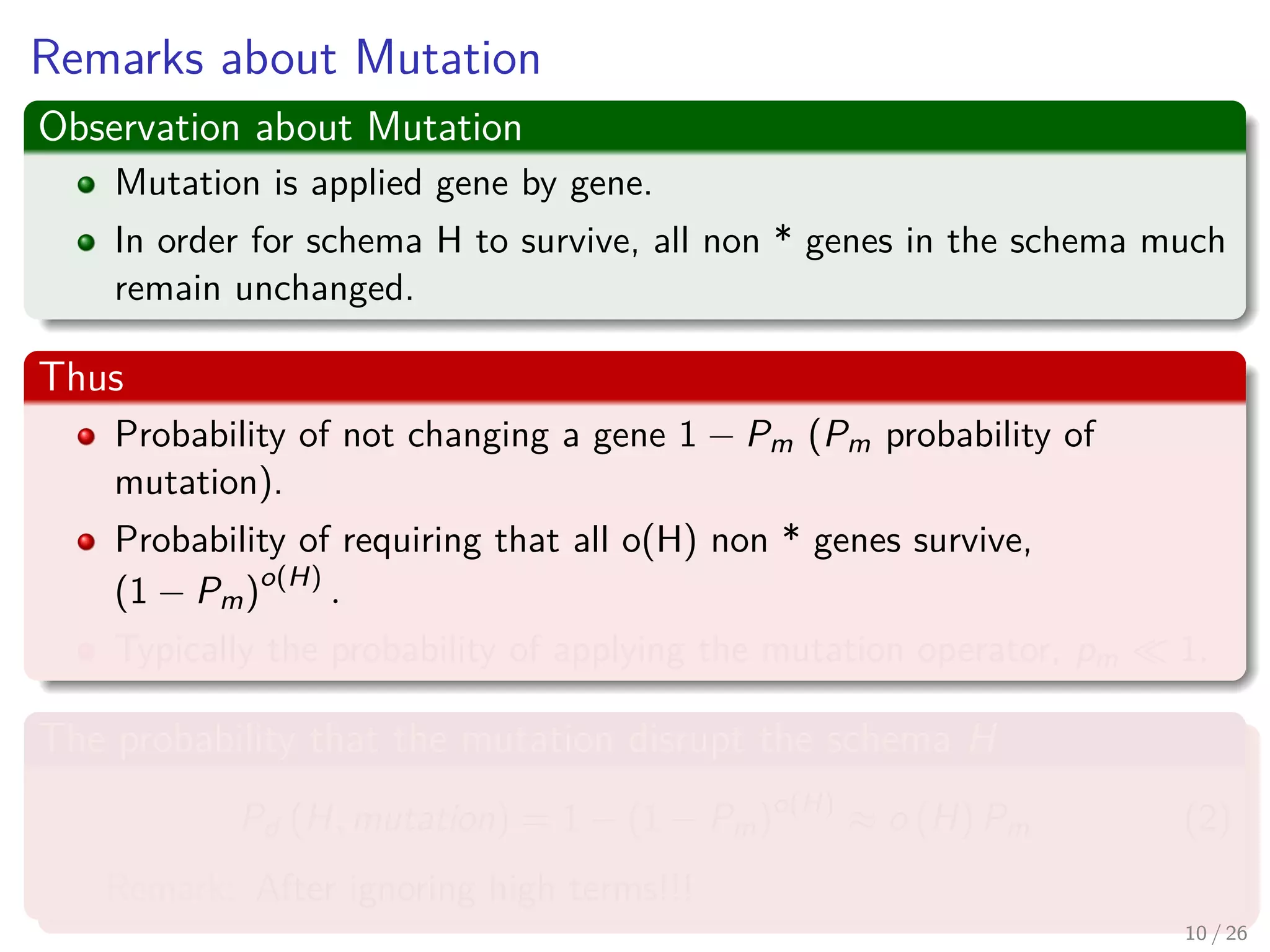
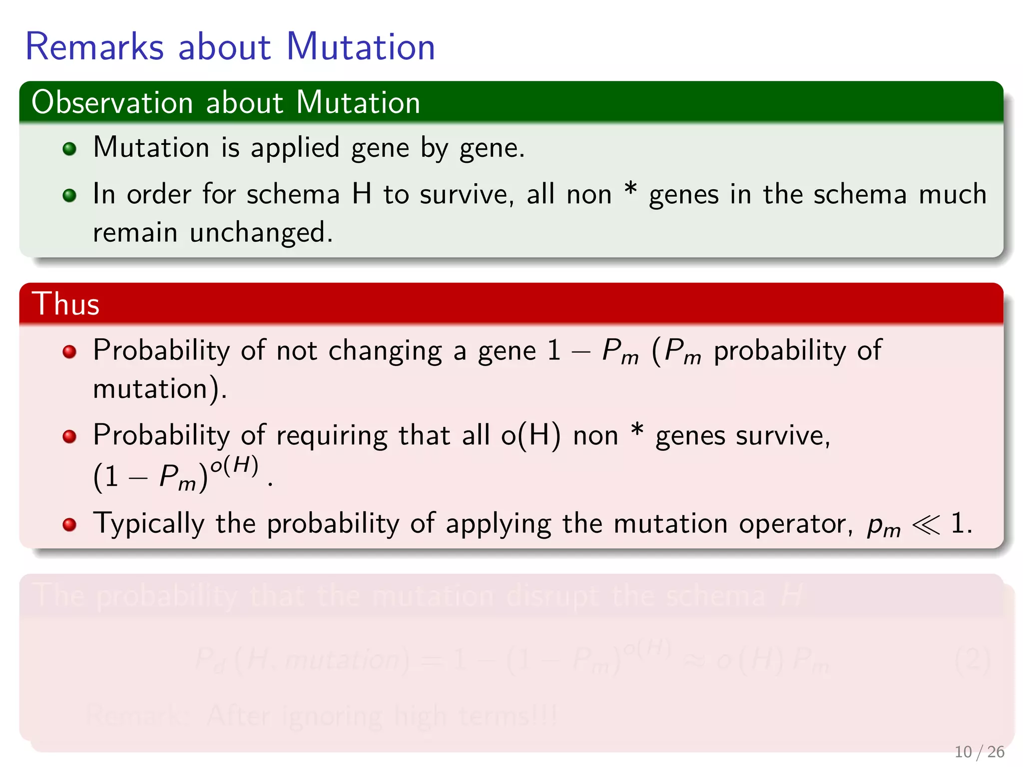
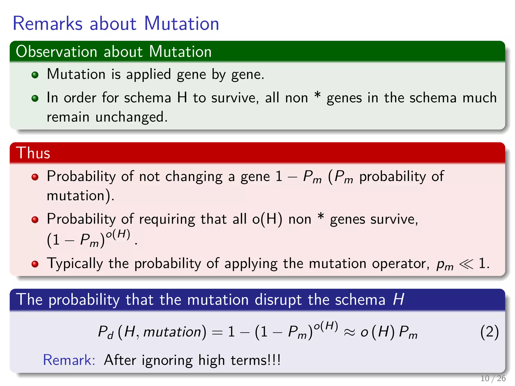
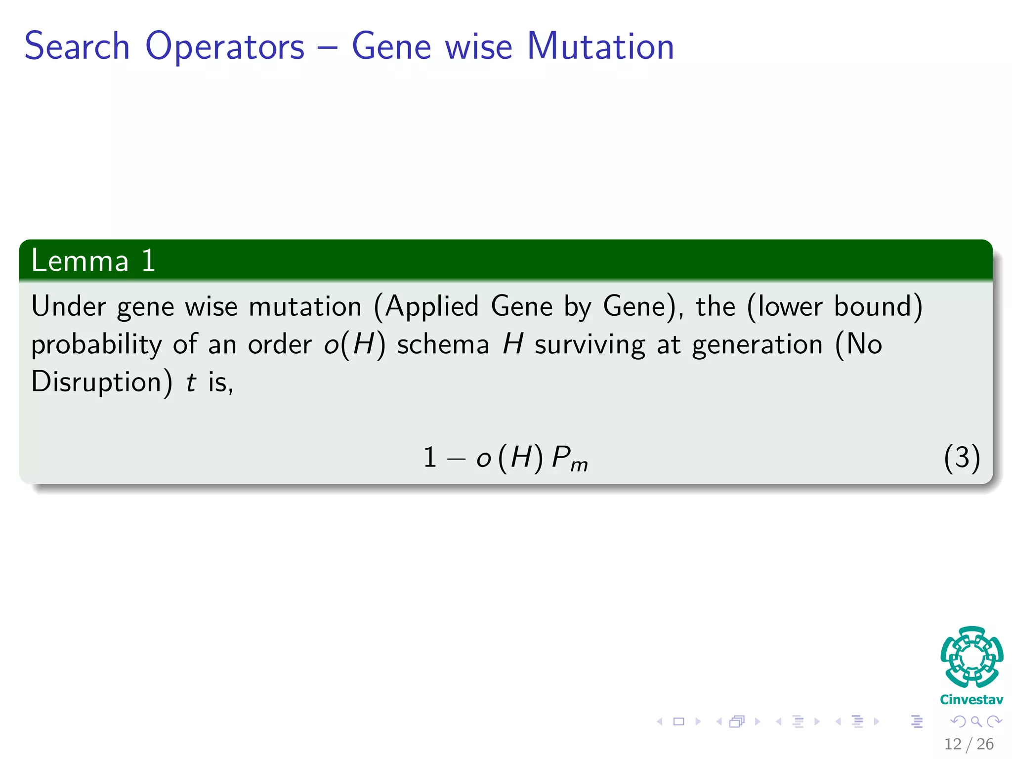
Discussion on mutation behaviors, preservation of genes, and the overall impact on schema.
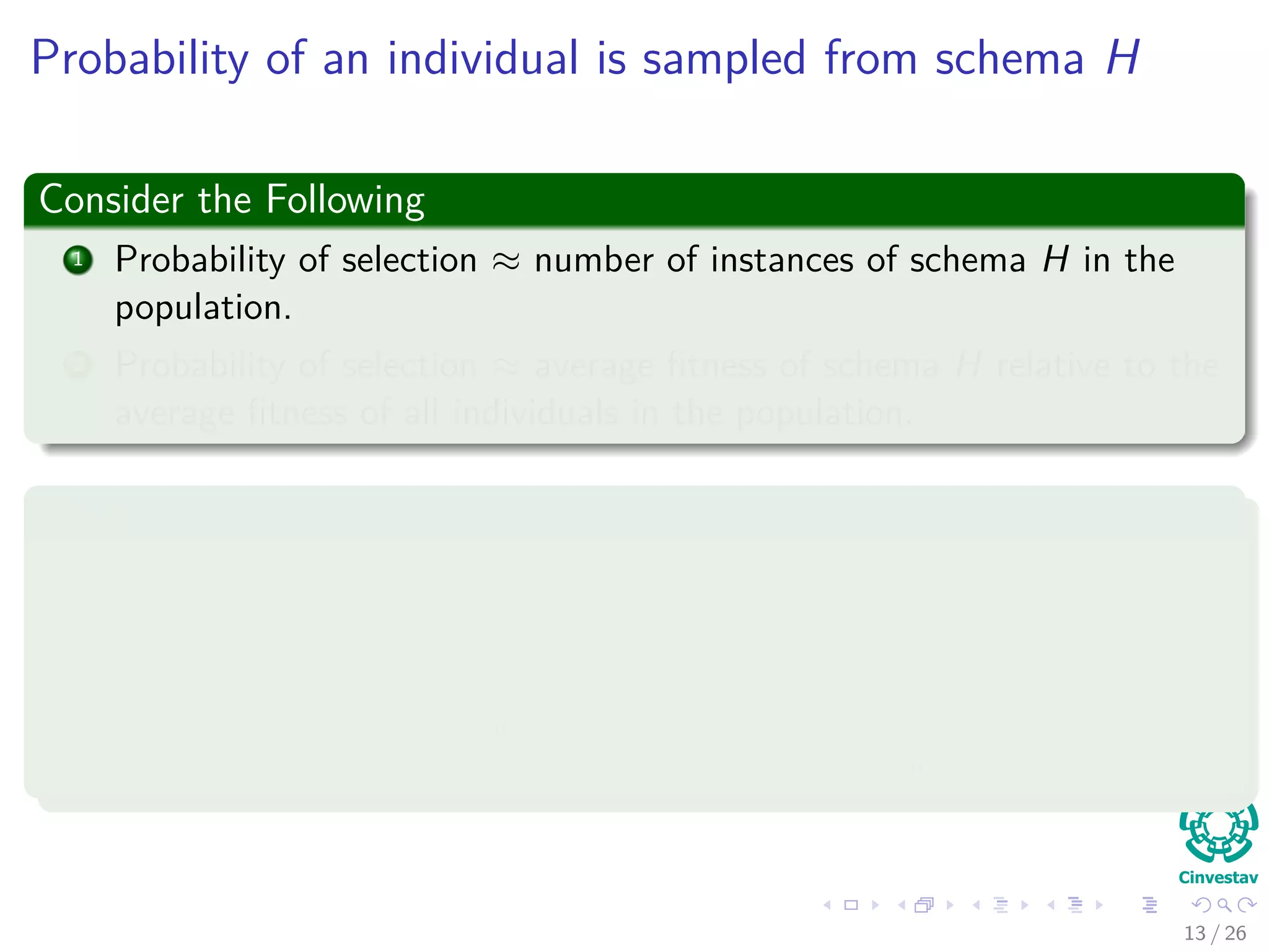
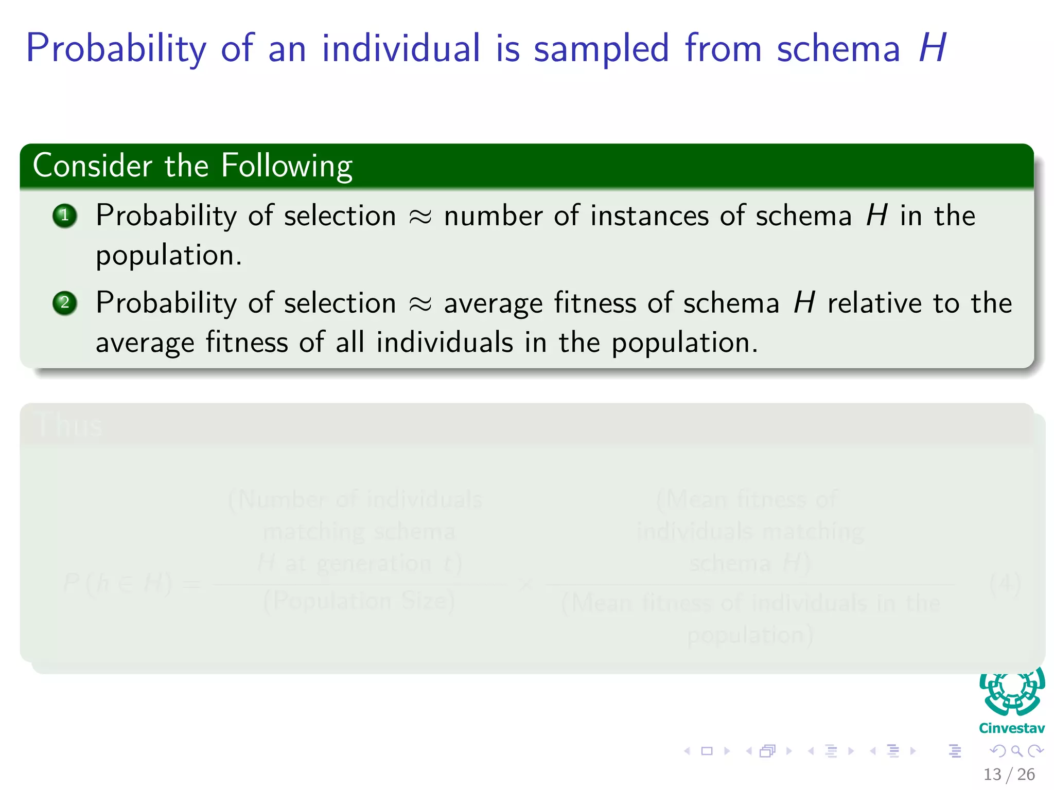
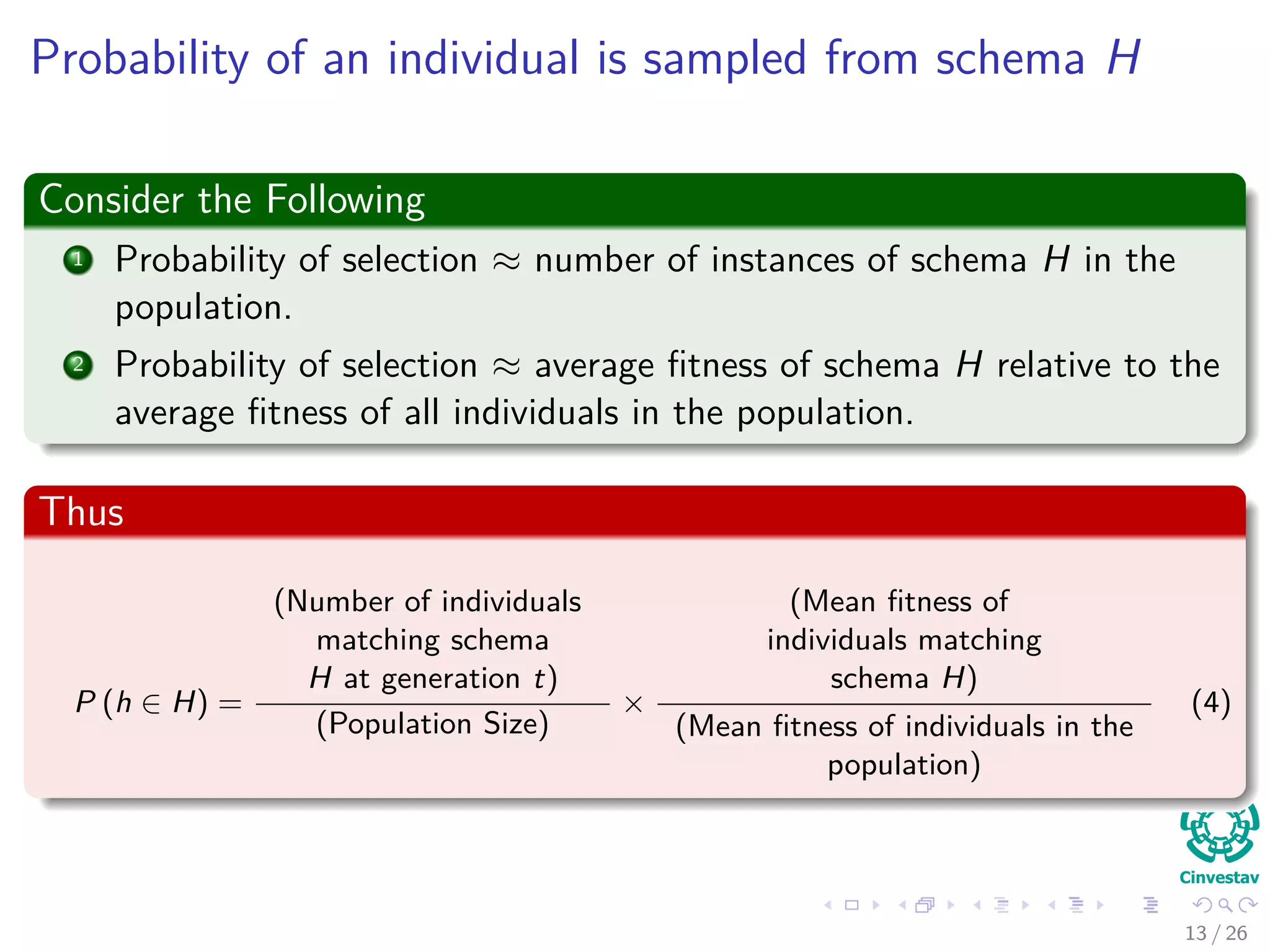
Probabilities for an individual originating from a specific schema, including fitness ratios.
Observations on the functioning of crossover as a search operator and the related schema survival. Introduction to the Schema Theorem and its generalizations with implications on schema behavior.
Discussion on the limitations and problems with the Schema Theorem and search operators.