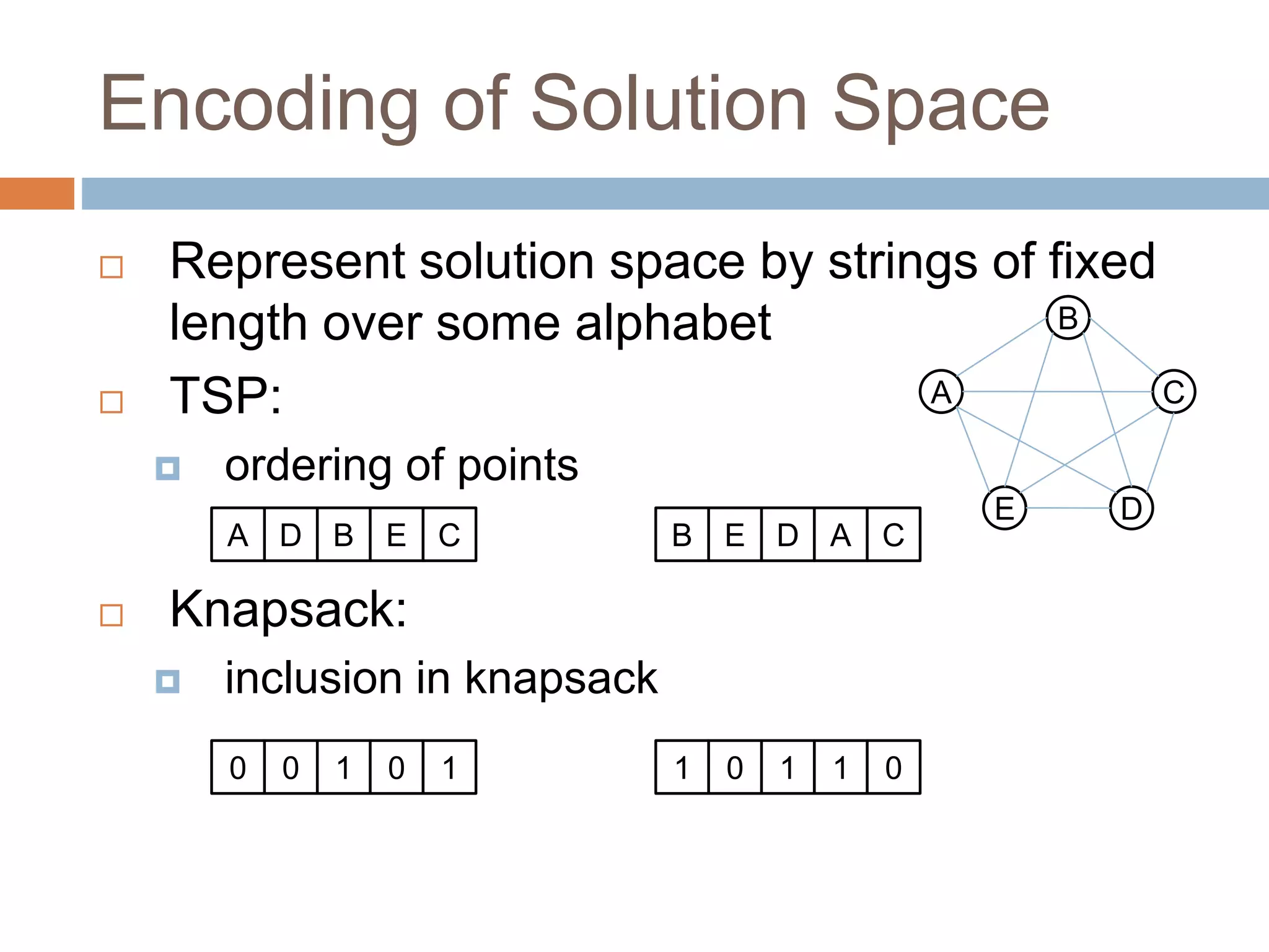
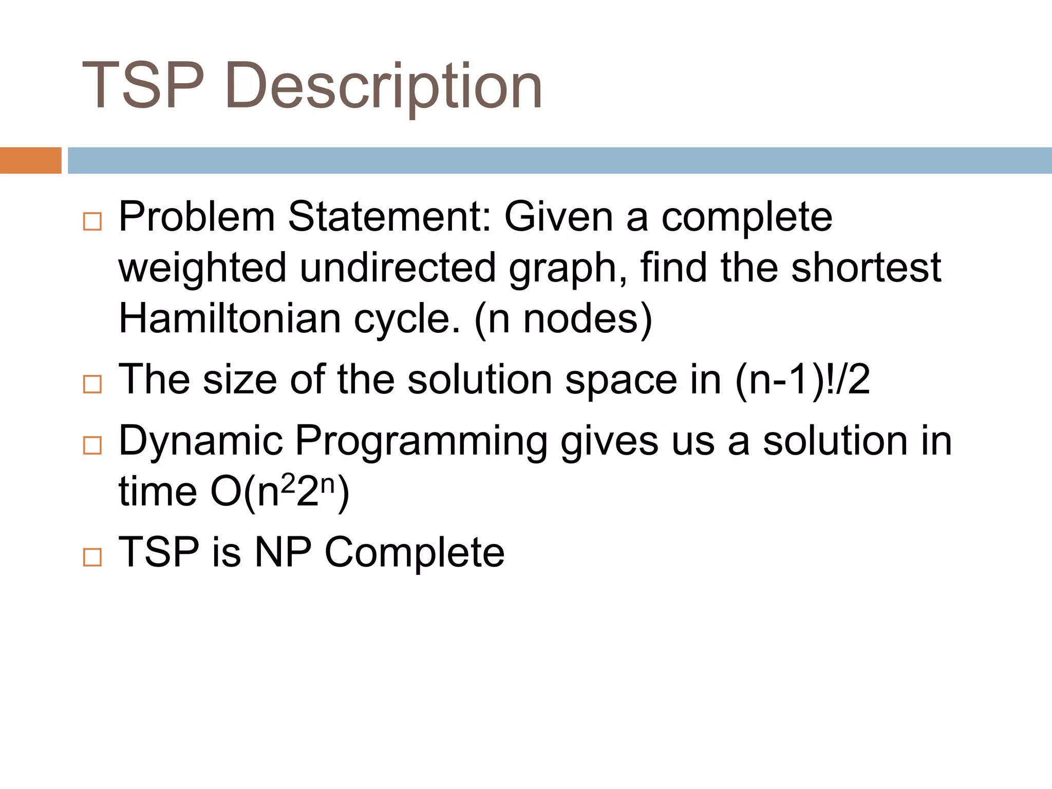
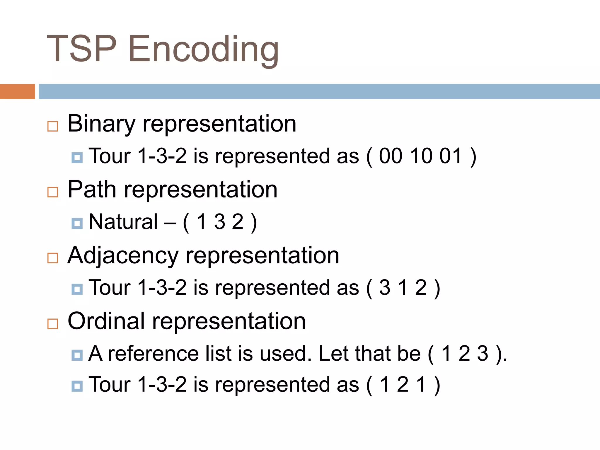
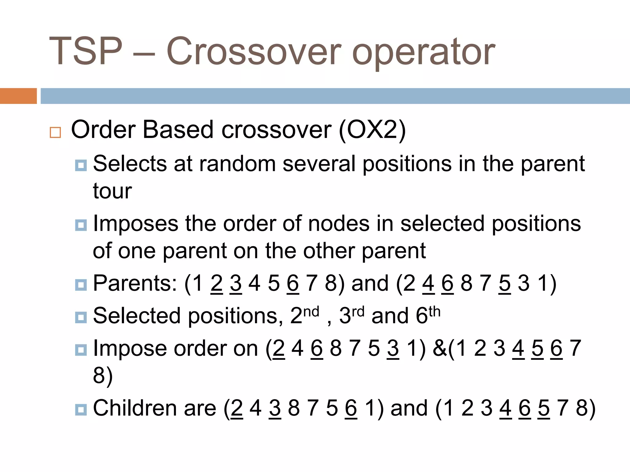
The document provides an overview of genetic algorithms, including their inspiration from evolution, the basic algorithm, why they work, strengths and weaknesses, and applications. It summarizes the encoding, selection, crossover, and mutation steps of the basic genetic algorithm. It also gives examples of genetic algorithms applied to the traveling salesman problem (TSP), including encoding solutions and crossover/mutation operators.

1. GENETIC
ALGORITHMS
Tanmay, Abhijit, Ameya, Saurabh

2. Inspiration - Evolution
• Natural Selection:
– “Survival of the Fittest”
– favourable traits become common and
unfavourable traits become uncommon in
successive generations
• Sexual Reproduction:
– Chromosomal crossover and genetic
recombination
– population is genetically variable
– adaptive evolution is facilitated
– unfavourable mutations are eliminated

3. Overview
 Inspiration
 The basic algorithm
 Encoding
 Selection
 Crossover
 Mutation
 Why Genetic Algorithms work ?
 Schemas
 Hyper-planes
 Schema Theorem
 Strengths and Weakness
 Applications
 TSP
 Conclusion

4. THE BASIC
ALGORITHM
Ameya Muley

5. Encoding of Solution Space
 Represent solution space by strings of fixed
length over some alphabet
 TSP:
 ordering of points
 Knapsack:
 inclusion in knapsack
A D B E C B E D A C
B
A C
E D
0 0 1 0 1 1 0 1 1 0

6. Selection
• Fitness function:
– f(x), x is a chromosome in the solution space
– f(x) may be:
• an well-defined objective function to be optimised
– e.g. TSP and knapsack
• a heuristic
– e.g. N-Queens
• Probability distribution for selection:
• Fitness proportional selection
 
 

 M
j j
i
i
x
f
x
f
x
X
P
1
)
(
)
(

7. Operators-Crossover and
Mutation
• Crossover:
– Applied with high probability
– Position for crossover on the two parent chromosomes randomly
selected
– Offspring share characteristics of well-performing parents
– Combinations of well-performing characteristics generated
• Mutation:
– Applied with low probability
– Bit for mutation randomly selected
– New characteristics introduced into the population
– Prevents algorithm from getting trapped into a local optimum

8. The Basic Algorithm
1. Fix population size M
2. Randomly generate M strings in the solution space
3. Observe the fitness of each chromosome
4. Repeat:
1. Select two fittest strings to reproduce
2. Apply crossover with high probability to produce offspring
3. Apply mutation to parent or offspring with low probability
4. Observe the fitness of each new string
5. Replace weakest strings of the population with the
offspring
until
i. fixed number of iterations completed, OR
ii. average/best fitness above a threshold, OR
iii. average/best fitness value unchanged for a fixed number of
consecutive iterations

9. Example
• Problem specification:
– string of length 4
– two 0’s and two 1’s
– 0’s to the right of the 1’s
• Solution space:
• Fitness function (heuristic):
– f(x) = number of bits that match the ones in the solution
• Initialization (M = 4):
0 0 1 1
 4
1
,
0
1 0 0 0 1
)
( 
A
f
0 1 0 0 1
)
( 
B
f
0 1 0 1 2
)
( 
C
f
0 0 1 0 3
)
( 
D
f
75
.
1

av
f
0 1 0 1
0 0 1 0
0 1 0 0
0 0 1 1
1
)
( 
X
f
4
)
( 
Y
f
0 1 0 0 0 1 1 0 2
)
( 
Z
f

10. Example (contd.)
 After iteration 1:
 After iteration 2:
0 1 0 1 2
)
( 
A
f
0 1 1 0 2
)
( 
B
f
0 0 1 0 3
)
( 
C
f
0 0 1 1 4
)
( 
D
f
75
.
2

av
f
0 1 0 1 2
)
( 
A
f
0 0 0 1 3
)
( 
B
f
0 0 1 0 3
)
( 
C
f
0 0 1 1 4
)
( 
D
f
3

av
f
0 1 0 1
0 0 1 0
0 1 1 0
0 0 0 1
2
)
( 
X
f
3
)
( 
Y
f

11. WHY GENETIC ALGORITHMS
WORK?
Tanmay Khirwadkar

12. Schemas
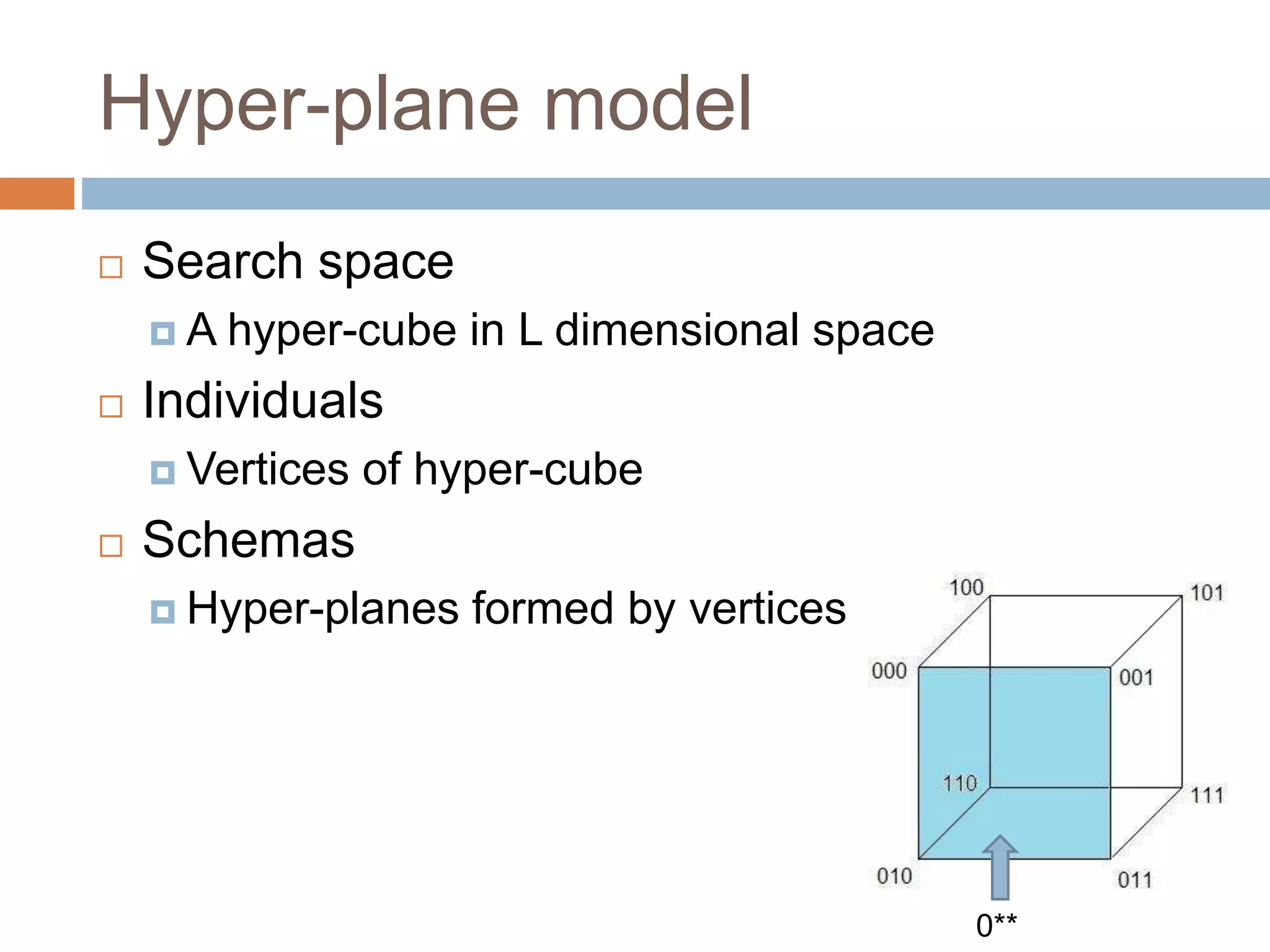
 Population
 Strings over alphabet {0,1} of length L
 E.g.
 Schema
 A schema is a subset of the space of all possible
individuals for which all the genes match the
template for schema H.
 Strings over alphabet {0,1,*} of length L
 E.g. }
11110
,
11010
,
10110
,
10010
{
]
10
*
*
1
[ 

H
10010

s

13. Hyper-plane model
 Search space
 A hyper-cube in L dimensional space
 Individuals
 Vertices of hyper-cube
 Schemas
 Hyper-planes formed by vertices
0**

14. Sampling Hyper-planes
 Look for hyper-planes (schemas) with good
fitness value instead of vertices (individuals) to
reduce search space
 Each vertex
 Member of 3L hyper-planes
 Samples hyper-planes
 Average Fitness of a hyper-plane can be
estimated by sampling fitness of members in
population
 Selection retains hyper-planes with good
estimated fitness values and discards others

15. Schema Theorem
 Schema Order O(H)
 Schema order, O(.) , is the number of non ‘*’ genes in
schema H.
 E.g. O(1**1*) = 2
 Schema Defining Length δ(H)
 Schema Defining Length, δ(H), is the distance
between first and last non ‘*’ gene in schema H
 E.g. δ(1**1*) = 4 – 1 = 3
 Schemas with short defining length, low order with
fitness above average population are favored by
GAs

16. Formal Statement
 Selection probability
 Crossover probability
 Mutation probability
 Expected number of members of a schema
)
,
(
)
,
(
)
,
(
))
1
,
(
(
t
H
f
t
H
f
t
H
m
t
H
m
E 

1
)
(
)
( 
 L
H
c
crossover p
h
P 
m
mutation p
H
h
P )
(
)
( 

))
(
1
)
(
1
(
)
,
(
)
,
(
)
,
(
)
1
,
(
( H
p
L
H
p
t
H
f
t
H
f
t
H
m
t
H
m
E m
c 







17. Why crossover and mutation?
 Crossover
 Produces new solutions while ‘remembering’ the
characteristics of old solutions
 Partially preserves distribution of strings across
schemas
 Mutation
 Randomly generates new solutions which cannot
be produced from existing population
 Avoids local optimum

18. STRENGTHS AND WEAKNESS
Abhijit Bhole

19. Area of application
GAs can be used when:
 Non-analytical problems.
 Non-linear models.
 Uncertainty.
 Large state spaces.

20. Non-analytical problems
 Fitness functions may not be expressed
analytically always.
 Domain specific knowledge may not be
computable from fitness function.
 Scarce domain knowledge to guide the
search.

21. Non-linear models
 Solutions depend on starting values.
 Non – linear models may converge to local
optimum.
 Impose conditions on fitness functions such as
convexity, etc.
 May require the problem to be approximated to
fit the non-linear model.

22. Uncertainty
 Noisy / approximated fitness functions.
 Changing parameters.
 Changing fitness functions.
 Why do GAs work? Because uncertainty is
common in nature.

23. Large state spaces
 Heuristics focus only on the immediate area of
initial solutions.
 State-explosion problem: number of states
huge or even infinite! Too large to be handled.
 State space may not be completely
understood.

24. Characteristics of GAs
 Simple, Powerful, Adaptive, Parallel
 Guarantee global optimum solutions.
 Give solutions of un-approximated form of
problem.
 Finer granularity of search spaces.

25. When not to use GA!
 Constrained mathematical optimization
problems especially when there are few
solutions.
 Constraints are difficult to incorporate into a
GA.
 Guided domain search is possible and
efficient.

26. PRACTICAL EXAMPLE - TSP
Saurabh Chakradeo

27. TSP Description
 Problem Statement: Given a complete
weighted undirected graph, find the shortest
Hamiltonian cycle. (n nodes)
 The size of the solution space in (n-1)!/2
 Dynamic Programming gives us a solution in
time O(n22n)
 TSP is NP Complete

28. TSP Encoding
 Binary representation
 Tour 1-3-2 is represented as ( 00 10 01 )
 Path representation
 Natural – ( 1 3 2 )
 Adjacency representation
 Tour 1-3-2 is represented as ( 3 1 2 )
 Ordinal representation
 A reference list is used. Let that be ( 1 2 3 ).
 Tour 1-3-2 is represented as ( 1 2 1 )

29. TSP – Crossover operator
 Order Based crossover (OX2)
 Selects at random several positions in the parent
tour
 Imposes the order of nodes in selected positions
of one parent on the other parent
 Parents: (1 2 3 4 5 6 7 8) and (2 4 6 8 7 5 3 1)
 Selected positions, 2nd , 3rd and 6th
 Impose order on (2 4 6 8 7 5 3 1) &(1 2 3 4 5 6 7
8)
 Children are (2 4 3 8 7 5 6 1) and (1 2 3 4 6 5 7 8)

30. TSP – Mutation Operators
 Exchange Mutation Operator (EM)
 Randomly select two nodes and interchange their
positions.
 ( 1 2 3 4 5 6 ) can become ( 1 2 6 4 5 3 )
 Displacement Mutation Operator (DM)
 Select a random sub-tour, remove and insert it in
a different location.
 ( 1 2 [3 4 5] 6 ) becomes ( 1 2 6 3 4 5 )

31. Conclusions
 Plethora of applications
 Molecular biology, scheduling, cryptography,
parameter optimization
 General algorithmic model applicable to a
large variety of classes of problems
 Another in the list of algorithms inspired by
biological processes – scope for more
parallels?
 Philosophical Implication:
 Are humans actually moving towards their global
optimum?

32. References
 Adaptation in Natural and Artificial Systems,
John H. Holland, MIT Press, 1992.
 Goldberg, D. E. 1989 Genetic Algorithms in
Search, Optimization and Machine Learning.
1st. Addison-Wesley Longman Publishing Co.,
Inc.
 Genetic Algorithms for the Travelling
Salesman Problem: A Review of
Representations and Operators, P. Larranaga
et al., University of Basque, Spain. Artificial
Intelligence Review, Volume 13, Number 2 /