The document discusses control systems and feedback control. It provides examples of regulatory control using a siphon water level control system. It describes open loop and closed loop control structures. Key signals in a feedback control loop are defined including the set point, error, control, disturbance, and noise signals. Time domain analysis in MATLAB is demonstrated including step response evaluations. Stability concepts are explained for different pole locations including real poles, imaginary poles, and complex poles. Effects of zeros and additional poles on stability are also covered. The document concludes with a brief discussion of specifying controller requirements.

1. CONTROL SYSTEMS
12-Apr-17
1
Eng. Mahmoud Hussein
RTECS

2. Control Objectives3

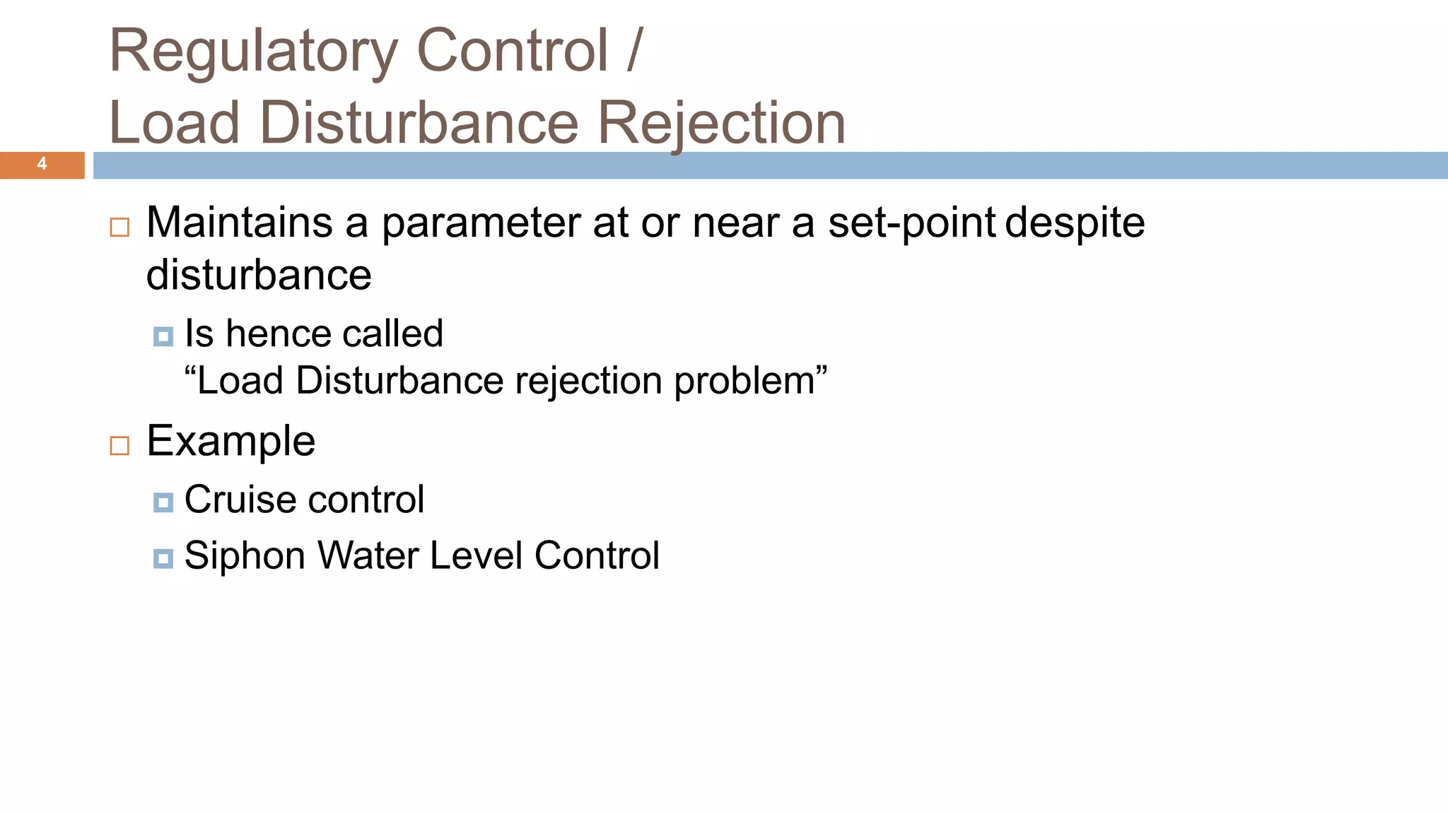
3. Regulatory Control /
Load Disturbance Rejection4
 Maintains a parameter at or near a set-point despite
disturbance
 Is hence called
“Load Disturbance rejection problem”
 Example
 Cruise control
 Siphon Water Level Control

4. Regulatory Control
Siphon Water Level Control5
 Principle of Operation
 OPEN
 If water level becomes low in the reservoir, the lever comes
down by the weight of floating ball and the ball of valve-
room rotating by the lever opens the flow way.
 CLOSE
 If water level becomes high in the reservoir, the lever comes
up by the buoyancy of floating ball and the ball of valve-
room rotating by the lever inside of valve closes the flow
way.

5. Regulatory Control
Siphon Water Level Control6
 Set point
 Normalizing the scale, the set point can be taken as a reference
 Desired signal = 0
 Output signal @ steady state = 0
 Control signal @ steady state = 0
 Disturbance
 Flushing the toilet

6. Servo Control / Setpoint Tracking Control /
Trajectory Control7
 Cause the plant output to follow the changing input command
as closely as possible
 Examples
 Remote control car
 Automatic parking control

7. Servo Control / Tracking Control Automatic
Parking Control8

8. Control Structures9

9. Open Loop Control
10

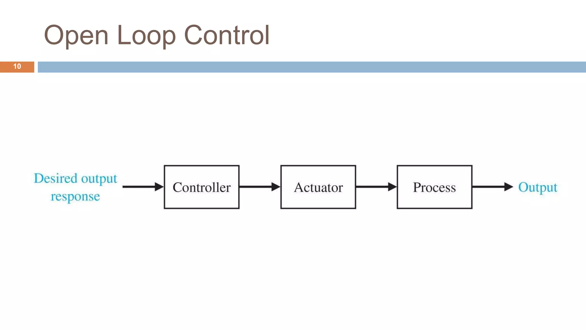
10. Open Loop Control
11
 Characteristics
 Highly sensitive to extraneous disturbances
 Highly sensitive to parametrical variation in the process
 TypicalApplications
 Stepper motor
 Motor with a worm gear (very high reduction ratio)
 Electric toaster

11. Closed Loop Control
(Feedback Control)12
Gc(s)
Controller
  n
sensor
noise

w load disturbance

Gprocess(s)
u
control
y
output
r
reference
input, or
set-point
e
 sensed
error
GActuator(s)
Actuator Process

12. Closed Loop Control
(Feedback Control)13
 Closed loop control strategy involves
 Measurement of the actual output,
 Comparison with the required reference value and
 Employing a suitable correction compensating for any deviation
Gc(s)
Controller
  n
sensor
noise

w load disturbance

u
control
y
output


r
reference
input, or
set-point
e
sensed
error
GActuator(s) Gprocess(s)
Actuator Process

13. Five Signals of Feedback Control Loop
14
 Set Point
 Desired output to be performed by the system
 constant for regulation control and
 variable for trajectory control
 Error signal
 The deviation between the desired behaviour and the system sensed output.
 Command/Control signal
 The signal generated from the controller
Gc(s)
Controller
  n
sensor
noise

w load disturbance
u
control
y
output

reference
input, or
set-point
r e
sensed
error
GActuator(s Gprocess(s))
Actuator Process

14. Five Signals of Feedback Control Loop
15
Gc(s)
  n
sensor
noise

 Disturbance
 A temporary change in environmental conditions that causes a
pronounced change in the system behaviour
 Low frequency deterministic measurable change
 Noise
 Random change of the signal at a high frequency
 Only statistically measurable
w load disturbance

Gprocess(s)
Process
u
control
y
output

reference
input, or
set-point
r e
sensed
error
GActuator(s)
Controller Actuator

15. Advantages of Feedback Control
16
 Speeds up the response
 Reduces steady-state error
 Reduces the sensitivity of a system to
 External disturbances
 Variations in its individual elements & components
 Improves stability

16. The Cost of Feedback
17
 Increased number of components and complexity
 Possibility of instability
 Whereas the open-loop system is stable, the closed-loop system
may not be always stable.

17. One DOF Feedback Controller18

18. One DOF Feedback Controller Block Diagram
19
Gc(s)
Controller
  n
sensor
noise

w load disturbance

Gp(s)
Plant
u
control
y
output
r
reference
input, or
set-point
e
 sensed
error
W(s)
Gp (s)
1GcGp (s)
N(s) 
GcGp (s)
1GcGp (s)
R(s) 
GcGp (s)
1GcGp (s)
Y (s)

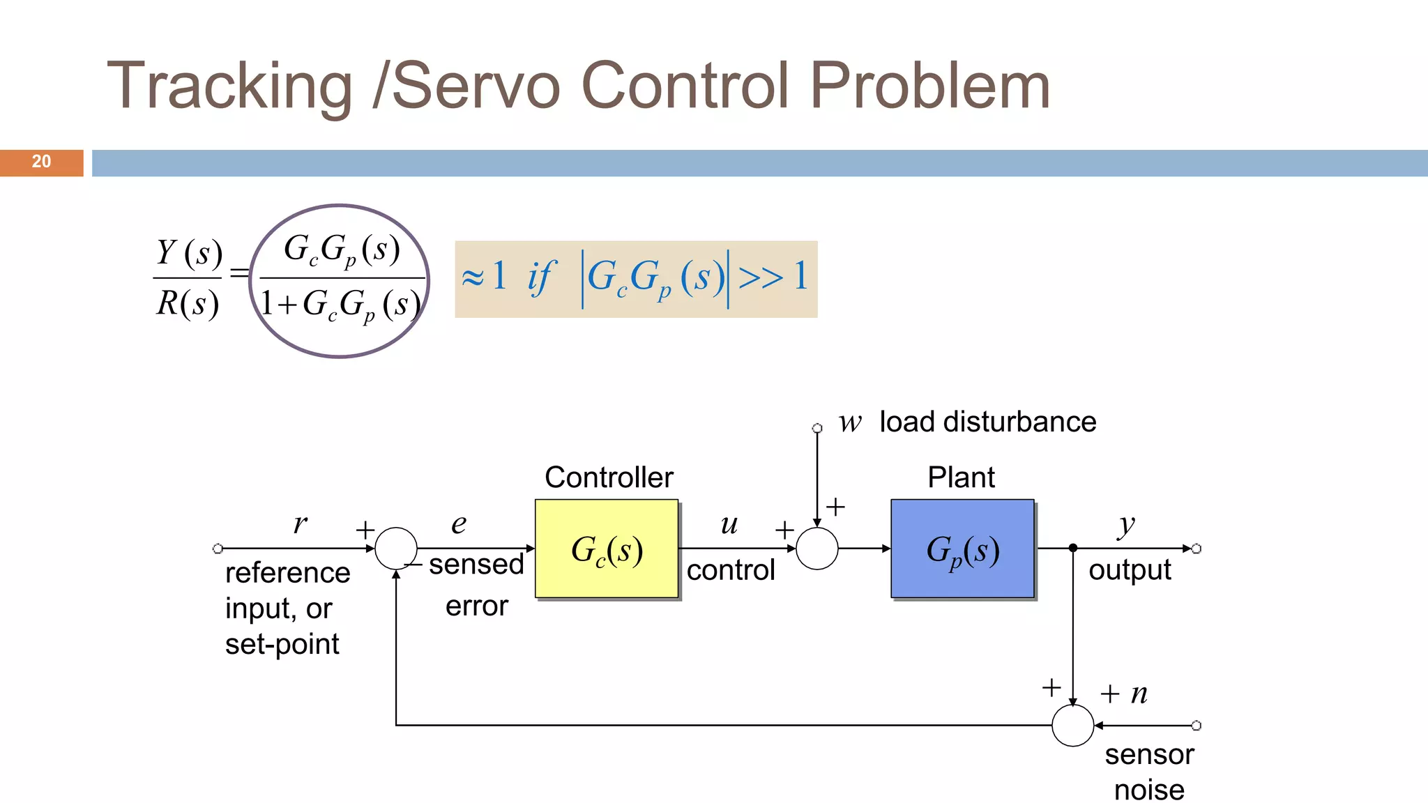
19. Tracking /Servo Control Problem
20
R(s)
GcGp (s)
1GcGp (s)
Y (s)

Gc(s)
Controller
  n
sensor
noise

w load disturbance

Gp(s)
Plant
u
control
y
output
r
reference
input, or
set-point
e
 sensed
error
1 if GcGp (s)  1

20. Disturbance Rejection Problem
21
Gc(s)
Controller
  n
sensor
noise

w load disturbance

Gp(s)
Plant
u
control
y
output
r
reference
input, or
set-point
e
 sensed
error
W(s)
Gp (s)
1GcGp (s)
Y(s)


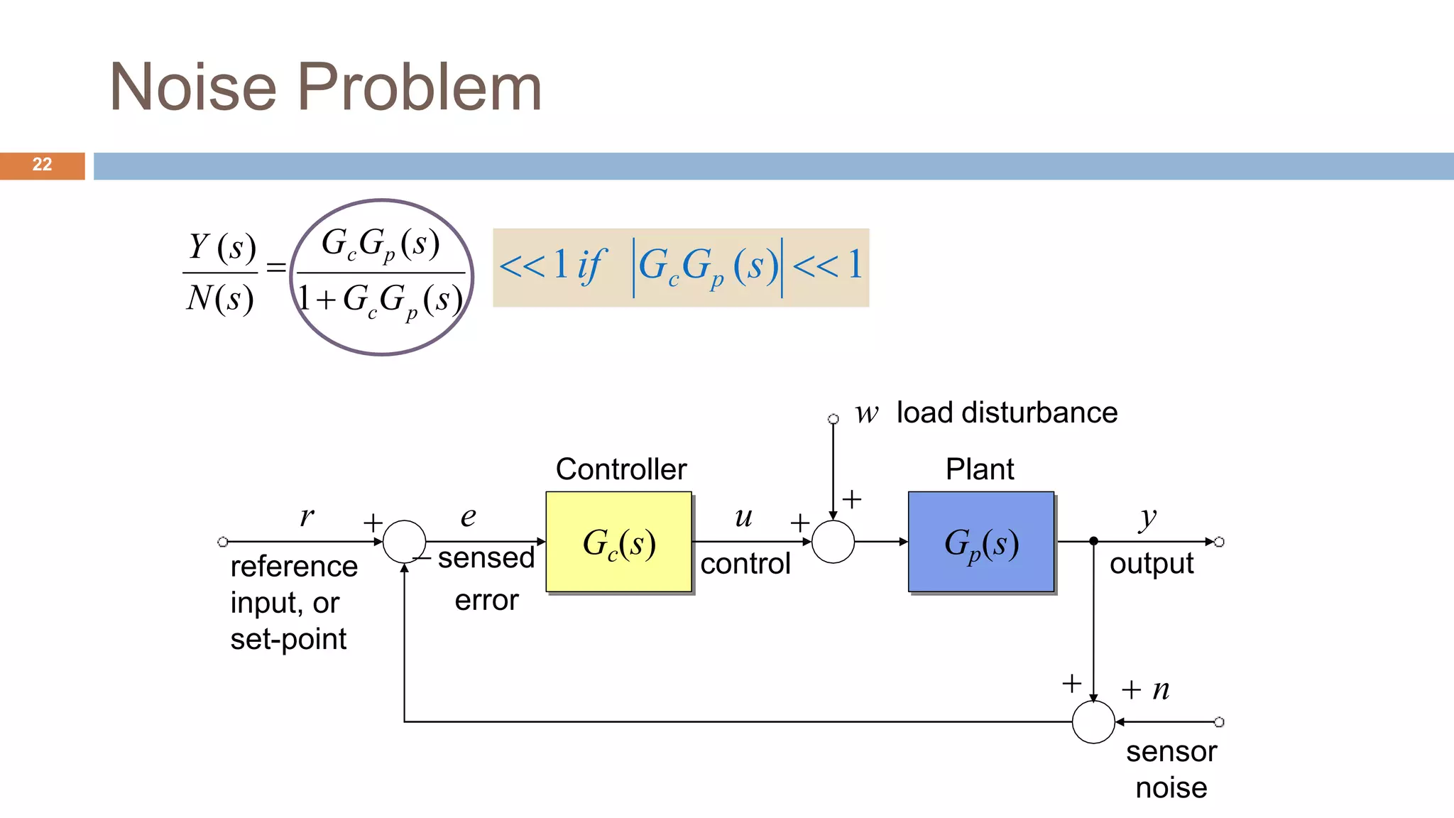
21. Noise Problem
22
Gc(s)
Controller
  n
sensor
noise

w load disturbance

Gp(s)
Plant
u
control
y
output
r
reference
input, or
set-point
e
 sensed
error
N(s) c p
GcGp (s)
1 G G (s)
Y (s)
 1if GcGp (s)  1

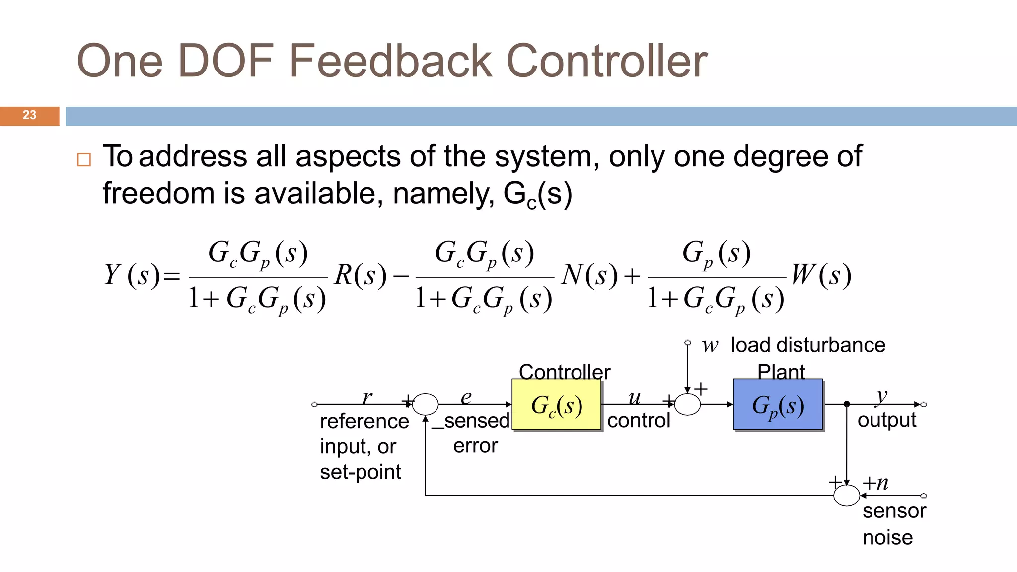
22. One DOF Feedback Controller
23
 To address all aspects of the system, only one degree of
freedom is available, namely, Gc(s)
W(s)
Gp (s)GcGp (s) GcGp (s)
1GcGp (s)
R(s)  N(s) 
1 GcGp (s) 1GcGp (s)
Y (s)
Gc(s)
Controller
 n
sensor
noise

w load disturbance

Gp(s)
Plant
u
control
y
output
r
reference
input, or
set-point
e
sensed
error

23.  Series Connection
 G=G2*G1
 where G1 and G2 are LTI objects (tf, ss, or zpk)
 Parallel Connection
 G=G1+G2
 where G1 and G2 are LTI objects (tf, ss, or zpk)
 Feedback Connection
 G=feedback(G,H,Sign)
 If Sign=-1, the negative feedback structure is indicated; negative feedbackis
the default
Modeling of Interconnected Block Diagrams in
Matlab24

24. Modeling of Interconnected Block Diagrams in
Matlab Example
 Where H(s) is a feeedback
block representing a first order
low pass filter with the aim of
sensor noise cancellation
 tf
 Create transfer function model, convert
to transfer function model
 feedback
 Feedback connection of two models
 Gp = tf( [1 7 24 24], [1 10 35 50 24] )
 Gc = tf( [10 5], [1 0] )
 H = tf( 1, [0.01, 1] )
 G_cl_loop = feedback( Gp*Gc, H, -1)
25
0.01s1
H (s)
s
1
10s 5
s3
 7s2
 24s 24
10s3
 35s2
 50s 24
Gc (s) 
Gp (s) 
s4

25. Time Domain Analysis in Matlab26

26. Step response evaluations with MATLAB
27
 step(G)
 %automatic draw of step response curves
 [y,t]=step(G)
 %evaluate the responses, but not drawn
 [y,t]=step(G,t_f)
 % final simulation time t_f setting
 y=step(G,t)
 %simulation on user defined time vector t

27. Unit Step Response in MATLAB
28
 OL_Sys = zpk([],[0 -6],25)
 CL_Sys = feedback(OL_Sys,1)
 figure
 step(CL_Sys);
 grid on
 stepinfo(CL_Sys)
R(s) + Y(s)25
s(s 6)

28. Unit Step Response in MATLAB
29
 RiseTime: 0.3711
 SettlingTime: 1.1887
 SettlingMin: 0.9083
 SettlingMax: 1.0948
 Overshoot: 9.4773
 Undershoot: 0
 Peak: 1.0948
 PeakTime: 0.7829
Step Response
Amplitude
0.2 0.4 0.6 0.8
Time(sec)
1 1.2 1.4 1.6
0
0
0.2
0.4
0.6
0.8
1
1.2
1.4
System: CL_Sys
Rise Time(sec ): 0.372
System: CL_Sys
Peak amplitude: 1.09
Overshoot (%): 9.47
At time (sec): 0.777 System: CL_Sys
Settling Time (sec): 1.19

29. Biological Feedback Control Example
30
 Regulation of glucose in the bloodstream through the
production of insulin and glucagon by the pancreas.

30. RTECS 2015 12-Apr-17

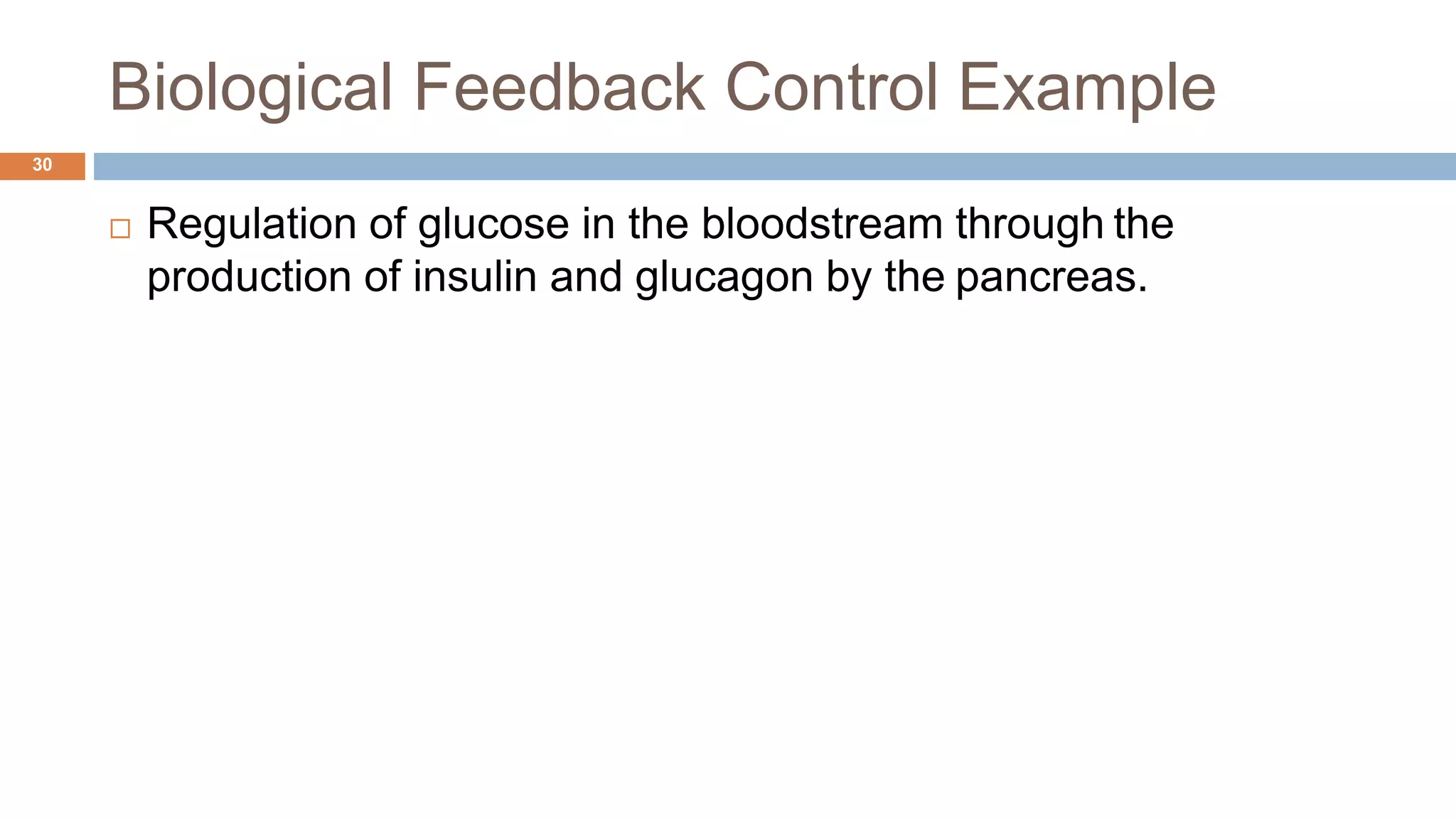
31. Biological Feedback Control Example
32
 Can you find out the components of the feedback control loop?
Control Device
Pancreas
Actuator
Insulin OR
Glucagon
Process
Liver
Actual Blood
Glucose Conc.
error
Sensor
Glucoreceptors
In Pancreas
+
-
Measured Blood
Glucose
Desired Blood
GlucoseConc.
(90 mg per100 mL ofblood)

32. Stability33
RTECS 2015

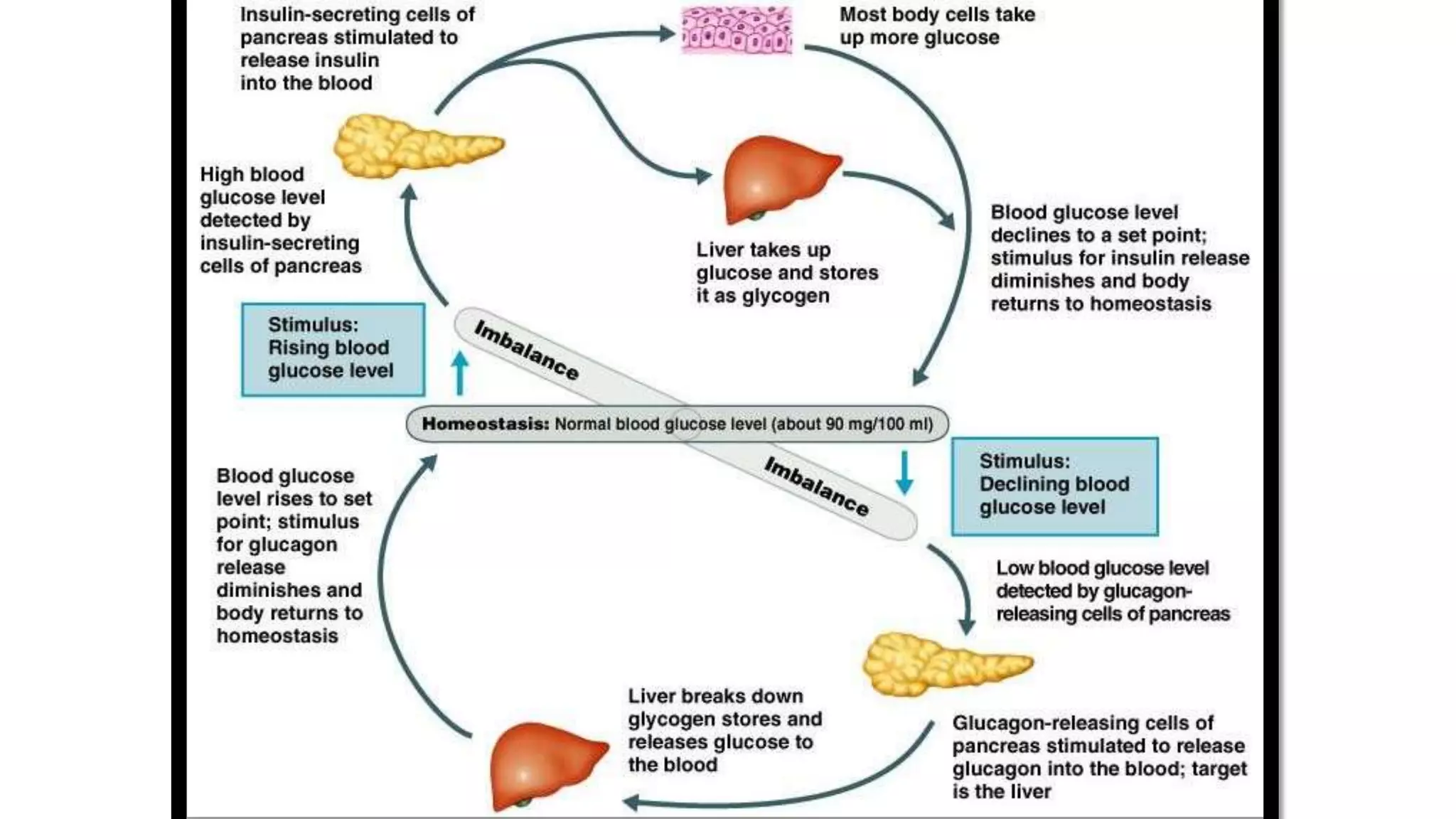
33. Simple Real Pole p = -
 The natural response is
of the form:
y(t )  K e t
K is given by the
initial condition
 Assuming K > 0:
34
if   0y(t)
if   0
t
 Location in s-domain:
Im(s)
if   0 if   0
Re(s)
Note: since  = 0, y(t) is located on
the real axis.

34. Simple Real Pole y(t )  Ke t
35
Note: Since  = 0, y(t) are located
on the real axis.
 Location in s-domain:
Im(s)
t
stable
Re(s)
stable
 Assuming K >0, if  >0:
y(t)
y(t) decays
t
• Effect of the value of  >0:
y(t) y(t) decay


35. Simple Real Pole y(t )  Ke t
 Assuming K >0, if  <0:
36
Note: Since  = 0, y(t) are located
on the real axis.
 Location in s-domain:
Im(s)
t
y(t)
unstable unstable
Re(s)
y(t) grows
t
• Effect of the value of  <0:
y(t) y(t) grow


36. Simple Real Pole p = 0
37
RTECS 2015
 The natural response is
of the form:
y(t)  B
B is given by the
initial condition
 Assuming B > 0:
y(t)
t
Note: since  = 0 and  = 0, y(t) is
located on the origin.
 Location in s-domain:
Im(s)
unstable
Re(s)

37. Simple Pair of Imaginary Poles
p = ± jd38
RTECS 2015
Re(s)
 The natural response is
of the form:
y(t )  Acos(d t ) Bsin( dt )
A and B are given by
the initial conditions
 Assuming A > 0, B > 0:
y(t)
t Note: since  = 0, y(t) is located on
the imaginary axis.
 Location in s-domain:
Im(s)
  0

38.  Assuming A > 0, B >0:
39
Re(s)
t
y(t)

y(t) oscillates
forever
t
Simple Pair of Imaginary Poles
y(t )  Acos(d t ) Bsin(dt )
• Effect of the value of  < 0:
y(t) y(t) oscillate
 Location in s-domain:
Im(s)
unstable
unstable
2

unstable
unstable
Note: In the case  = 0, the systemis
said unstable or critically stable.
RTECS 2015

39. Simple Pair of Complex Poles
p = - ±jd
d dAcos( t ) Bsin(  t )y(t )  et
 The natural response is
of the form:
A and B are given by
the initial conditions
40
RTECS 2015
if   0
 Location in s-domain:
Im(s)
if   0
if   0
 Assuming A >0, B > 0:
y(t)
if   0
t
stable unstable
Re(s)
stable unstable

40. Effects of Zeros
41
 A zero in the left half-plane
 Increases the overshoot if the zero is within a factor of 4 of the real
part of the complex poles. whereas it has very little influence on the
settling time.
 A zero in the right half-plane
 Depress the overshoot (and may causes an initial undershoot (=the
step response starts out in the wrong direction).

41. Effects of Additional Poles
42
 An additional pole in the left half plane
 increases the rise time significantly (=slows down the response) if
the extra pole is within a factor 4 of the real part of the complex
poles.
 If the extra real pole  is more than 6 times Re{p}, the effect is
negligible.

42. RTECS 201543

43. Well Behaved Signals44

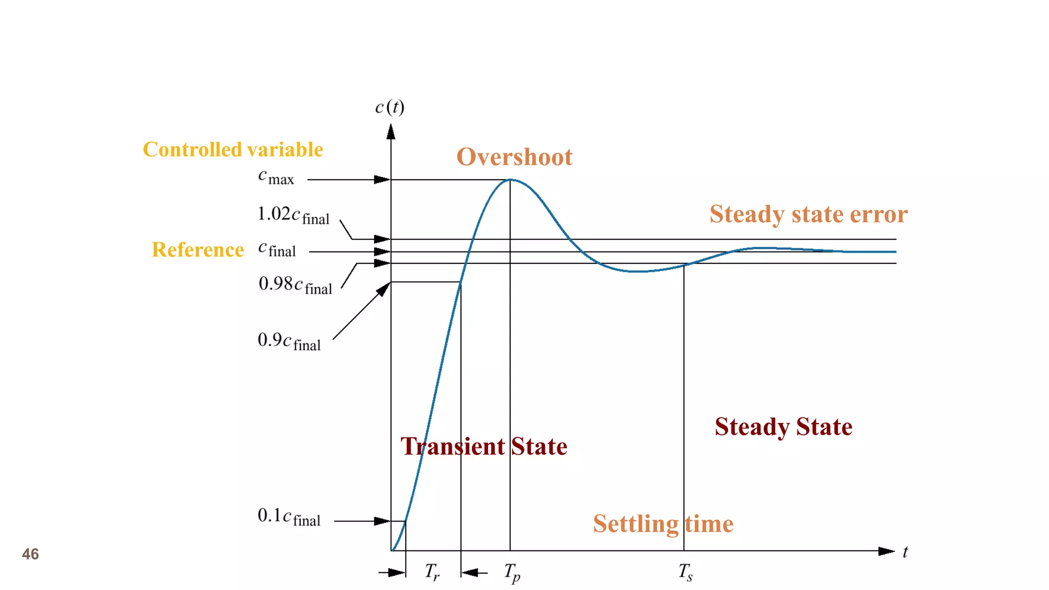
44. How To Specify Controller Requirements ?
45
 Step Input
 Specify the requirements on the response to a step reference signal
 Transient Response
 First part of system response when the output is still changing
 Steady State Response
 The final state for the system output

45. RTECS 201546
Settling time
OvershootControlled variable
Reference
Steady State
Transient State
Steady state error

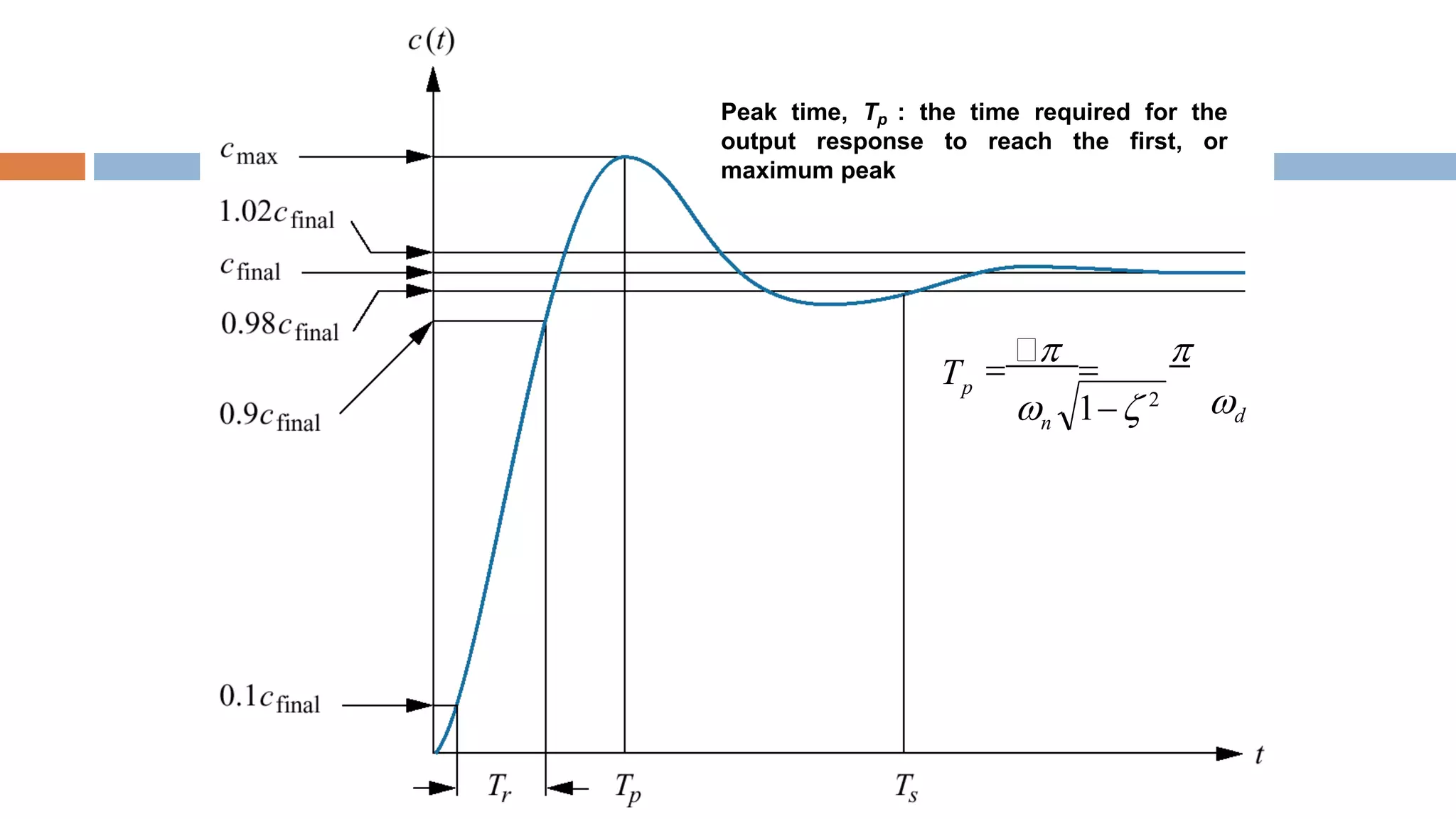
46. Delay time, Td : the time needed for the
output response to reach 50% of its final
value.

47. Rise time, Tr : the time taken for the output
response to go from 10% to 90% of its final
value.

48. Settling time, Ts : the time taken for the
output response to reach, and stay within
2% of its final output value
dn
s
 
4

4
T 

49. Peak time, Tp : the time required for the
output response to reach the first, or
maximum peak
dn
pT


 

 1 2

50. Percentage overshoot, %OS : the amount
of the output response overshoots the final
value at the peak time, expressed in
percentage of steady-state value
cfinal
c final
100%%OS 
cmax
1 2
%OS  e 100%
1 2
)
cmax
( /
 c(tp ) 1 e


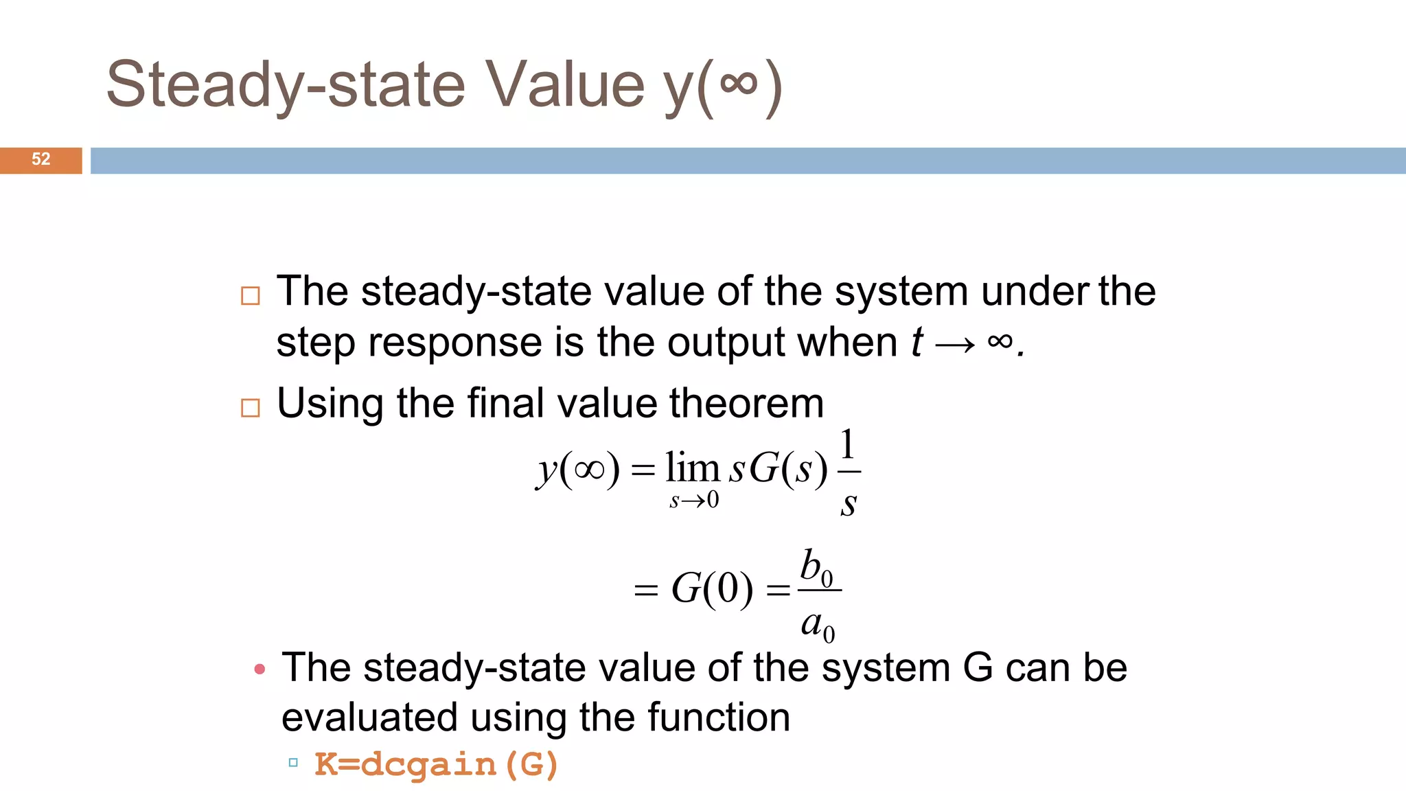
51. • The steady-state value of the system G can be
evaluated using the function
▫ K=dcgain(G)
Steady-state Value y(∞)
52
 The steady-state value of the system under the
step response is the output when t → ∞.
 Using the final value theorem
a0
s
y()  lim sG(s)
1
s0
 G(0) 
b0

52. Laplace Transform Method
53
 Inverse Laplace transformation is used to obtain the output
signal in the time domain
 Symbolic Toolbox of MATLAB

53. Laplace Transform Method Example
54
s4
u(t)  2 2e3t
sin(2t)
 For the transfer function G(s) and the input u(t),
obtain the output y(t)
 Hint
 Laplace command: laplace
 Inverse Laplace command: i laplace
 7s3
17s2
17s 6
s3
 7s2
3s  4
G(s) 

54. RTECS