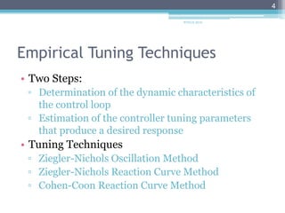
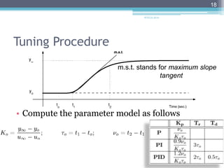
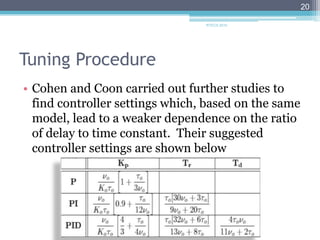
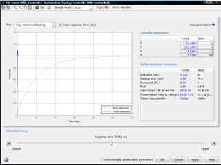
Tuning PID Controllers
Eng. Mahmoud Hussein
RTECS 2010
1
RTECS 2010
1
Gc(s)
Controller
+
+ n
sensor
noise
+
w load disturbance
+
Gp(s)
Plant
u
control
y
output
+
-
r
reference
input, or
set-point
e
sensed
error
RTECS 2010
2
Analytical Vs. Empirical Techniques
• Analytical Tuning Techniques
▫ Frequency response analysis
• Empirical Tuning Techniques
▫ On-line tuning after the control system is installed
▫ Computer simulation
RTECS 2010
3
Empirical Tuning Techniques
• Two Steps:
▫ Determination of the dynamic characteristics of
the control loop
▫ Estimation of the controller tuning parameters
that produce a desired response
• Tuning Techniques
▫ Ziegler-Nichols Oscillation Method
▫ Ziegler-Nichols Reaction Curve Method
▫ Cohen-Coon Reaction Curve Method
RTECS 2010
4
Z-N Closed Loop Method
Z-N Continuous Cycling Method
By Ziegler and Nichols (1942)
RTECS 2010
5
Quarter Decay Ratio Response By
Ultimate Gain
• Use the proportional controller to force
sustained oscillations.
• Goal is to determine ultimate gain and ultimate
period of oscillation of the control loop
RTECS 2010
6
Quarter Decay Ratio Response By
Ultimate Gain
• Ziegler-Nichols method specifies a decay ratio of
one-fourth (1/4)
• Decay ratio = ratio of the amplitudes of two
successive oscillations
RTECS 2010
7
Tuning Procedure
• Set the true plant under proportional control,
with a very small gain
• Increase the gain until the loop starts oscillating
▫ Note that linear oscillation is required and that it
should be detected at the controller output.
• Record the controller critical gain (ultimate
gain) Kp = Kc (Ku) and the oscillation period of
the controller output, Pc (Pu).
RTECS 2010
8
Tuning Procedure
• Calculate the parameters according to the
following formulas
RTECS 2010
9
Controlle
r Type
Proportional
Gain (Kp)
Integral
Time (tI)
Derivative
Time (tD)
P-only Ku/2 - -
PI Ku/2.2 Pu/1.2 -
PID Ku/1.7 Pu/2 Pu/8
Example
• Consider the given plant
▫ Find the parameters of a PID controller using the
Z-N oscillation method.
▫ Obtain a graph of the response to a unit step input
reference.
RTECS 2010
10
 3
1
1
)(
+

s
sGp
Example Solution
• Applying the procedure we find
▫ Kc = 8 and ωc = 3
• Hence, from Table we have
▫ Kp = 4.8
▫ Tr = 1.81
▫ Td = 0.45
• Try the same procedure for the second order
system
RTECS 2010
11
 2
1
1
)(
+

s
sGp
Drawbacks
• Time-consuming
▫ If the process dynamics are slow
• The process is pushed to the stability limits
▫ Risk of plant damage
• For first-order and second-order model without
time delays the ultimate gain does not exist
▫ Because the closed-loop system is stable for all
values of Kp. However, in practice, it is unusual
for a control loop not to have an ultimate gain.
RTECS 2010
12
RTECS 2010
13
Tuning Procedure
• Same procedure as Z-N closed loop method
• TLC tuning values tend to reduce oscillatory
effects and improves robustness.
RTECS 2010
14
Z-N Open-loop Method
RTECS 2010
15
Process Reaction Curve
• From the open loop step response, the system
dynamics can be determined
• The controller settings are based on the open-
loop step response, or in other words, the
process reaction curve
RTECS 2010
16
Tuning Procedure
• With the plant in open loop, take the plant
manually to a normal operating point
▫ Say that the plant output settles at y(t) = y0 for a
constant plant input u(t) = u0.
• At an initial time, t0, apply a step change to the
plant input, from u0 to u
▫ This should be in the range of 10 to 20% of full
scale
• Record the plant output until it settles to the
new operating point. Assume you obtain the
curve shown on the next slide.
RTECS 2010
17
Tuning Procedure
RTECS 2010
18
• Compute the parameter model as follows
m.s.t. stands for maximum slope
tangent
RTECS 2010
19
Tuning Procedure
• Cohen and Coon carried out further studies to
find controller settings which, based on the same
model, lead to a weaker dependence on the ratio
of delay to time constant. Their suggested
controller settings are shown below
RTECS 2010
20
Simulink Control Design 3.0
RTECS 2010
21
PID Controller Block
▫ PID_Controller_Automated_Tuning.mdl
RTECS 2010
22
Initial PID Design
RTECS 2010
23
Adjusting Response Time To Tune
Parameters
RTECS 2010
24

05 tuning.pid.controllers

  • 1.
    Tuning PID Controllers Eng.Mahmoud Hussein RTECS 2010 1 RTECS 2010 1 Gc(s) Controller + + n sensor noise + w load disturbance + Gp(s) Plant u control y output + - r reference input, or set-point e sensed error
  • 2.
  • 3.
    Analytical Vs. EmpiricalTechniques • Analytical Tuning Techniques ▫ Frequency response analysis • Empirical Tuning Techniques ▫ On-line tuning after the control system is installed ▫ Computer simulation RTECS 2010 3
  • 4.
    Empirical Tuning Techniques •Two Steps: ▫ Determination of the dynamic characteristics of the control loop ▫ Estimation of the controller tuning parameters that produce a desired response • Tuning Techniques ▫ Ziegler-Nichols Oscillation Method ▫ Ziegler-Nichols Reaction Curve Method ▫ Cohen-Coon Reaction Curve Method RTECS 2010 4
  • 5.
    Z-N Closed LoopMethod Z-N Continuous Cycling Method By Ziegler and Nichols (1942) RTECS 2010 5
  • 6.
    Quarter Decay RatioResponse By Ultimate Gain • Use the proportional controller to force sustained oscillations. • Goal is to determine ultimate gain and ultimate period of oscillation of the control loop RTECS 2010 6
  • 7.
    Quarter Decay RatioResponse By Ultimate Gain • Ziegler-Nichols method specifies a decay ratio of one-fourth (1/4) • Decay ratio = ratio of the amplitudes of two successive oscillations RTECS 2010 7
  • 8.
    Tuning Procedure • Setthe true plant under proportional control, with a very small gain • Increase the gain until the loop starts oscillating ▫ Note that linear oscillation is required and that it should be detected at the controller output. • Record the controller critical gain (ultimate gain) Kp = Kc (Ku) and the oscillation period of the controller output, Pc (Pu). RTECS 2010 8
  • 9.
    Tuning Procedure • Calculatethe parameters according to the following formulas RTECS 2010 9 Controlle r Type Proportional Gain (Kp) Integral Time (tI) Derivative Time (tD) P-only Ku/2 - - PI Ku/2.2 Pu/1.2 - PID Ku/1.7 Pu/2 Pu/8
  • 10.
    Example • Consider thegiven plant ▫ Find the parameters of a PID controller using the Z-N oscillation method. ▫ Obtain a graph of the response to a unit step input reference. RTECS 2010 10  3 1 1 )( +  s sGp
  • 11.
    Example Solution • Applyingthe procedure we find ▫ Kc = 8 and ωc = 3 • Hence, from Table we have ▫ Kp = 4.8 ▫ Tr = 1.81 ▫ Td = 0.45 • Try the same procedure for the second order system RTECS 2010 11  2 1 1 )( +  s sGp
  • 12.
    Drawbacks • Time-consuming ▫ Ifthe process dynamics are slow • The process is pushed to the stability limits ▫ Risk of plant damage • For first-order and second-order model without time delays the ultimate gain does not exist ▫ Because the closed-loop system is stable for all values of Kp. However, in practice, it is unusual for a control loop not to have an ultimate gain. RTECS 2010 12
  • 13.
  • 14.
    Tuning Procedure • Sameprocedure as Z-N closed loop method • TLC tuning values tend to reduce oscillatory effects and improves robustness. RTECS 2010 14
  • 15.
  • 16.
    Process Reaction Curve •From the open loop step response, the system dynamics can be determined • The controller settings are based on the open- loop step response, or in other words, the process reaction curve RTECS 2010 16
  • 17.
    Tuning Procedure • Withthe plant in open loop, take the plant manually to a normal operating point ▫ Say that the plant output settles at y(t) = y0 for a constant plant input u(t) = u0. • At an initial time, t0, apply a step change to the plant input, from u0 to u ▫ This should be in the range of 10 to 20% of full scale • Record the plant output until it settles to the new operating point. Assume you obtain the curve shown on the next slide. RTECS 2010 17
  • 18.
    Tuning Procedure RTECS 2010 18 •Compute the parameter model as follows m.s.t. stands for maximum slope tangent
  • 19.
  • 20.
    Tuning Procedure • Cohenand Coon carried out further studies to find controller settings which, based on the same model, lead to a weaker dependence on the ratio of delay to time constant. Their suggested controller settings are shown below RTECS 2010 20
  • 21.
    Simulink Control Design3.0 RTECS 2010 21
  • 22.
    PID Controller Block ▫PID_Controller_Automated_Tuning.mdl RTECS 2010 22
  • 23.
  • 24.
    Adjusting Response TimeTo Tune Parameters RTECS 2010 24