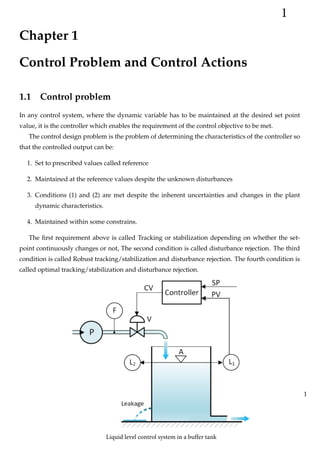
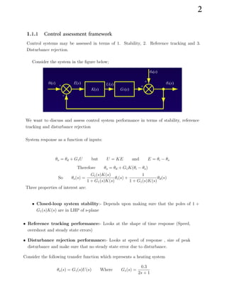
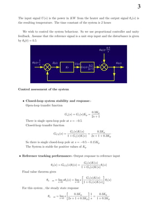
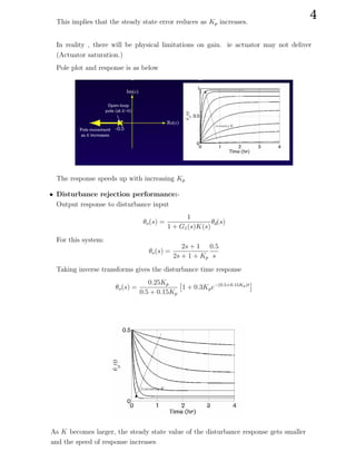
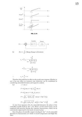
The document discusses control system assessment in terms of stability, reference tracking, and disturbance rejection. It provides an example of assessing the performance of a heating system controlled with a proportional controller. The key points are:
1) Closed-loop stability depends on the poles of the closed-loop transfer function being in the left half of the s-plane.
2) Reference tracking performance is assessed by examining the system response and steady-state error.
3) Disturbance rejection performance looks at the speed and size of the system response to disturbances.
![Characteristics of + + controller
€
€
‚ƒ ‚
„ †‡
ˆ
‰
†
†
Š‹ Œ
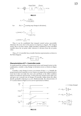
1.5.3 Proportional + Integral + Derivative Controller
Mode
[+ + Mode]
1
T S
i
Kp 1 +
P S
( )
E S
( )
+ d
T S
16](https://image.slidesharecdn.com/inno2019emt4203controliichap1controlactions-231222092847-1a48ee43/85/Inno2019_EMT4203_CONTROL_II_Chap1_Control-Actions-pdf-17-320.jpg)