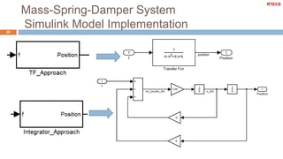
1) The document discusses physical system modelling and modelling of mechanical systems. It defines a physical system and classifies systems as static or dynamic. 2) For dynamic systems, it describes representing them mathematically using differential equations and introduces modelling basic mechanical elements like mass, springs and dampers. 3) An example is given of modelling a mass-spring-damper system using both an integrator approach and transfer function approach. The simulink model of the system is also demonstrated. 4) Vehicle suspension systems are described as an example of modelling a real mechanical system, with the quarter-car model introduced.

1. PHYSICAL SYSTEM MODELLING
MECHANICAL SYSTEMS
Eng. Mahmoud Hussein
28-Feb-17
RTECS 2015 1
RTECS_2017

2. Modelling the Plant
Physical System Modelling3
RTECS

3. Definition of System
23
 From engineering point of view, a system is defined as an
interconnection of many components that act together to
perform a certain objective
 Automobile
 Machine tool
 Robot
RTECS

4. Physical Systems Classification
24
Physical
System
Static System Dynamic
System
RTECS

5. Static System
25
 Output of the system depends only on the current input
 The system has no memory
RTECS

6. Dynamic System
26
 Output of the system depends on the current input as well as
previous inputs/outputs
 The system has internal memory
A dynamic system can be represented mathematically
using differential equations
RTECS

7. Dynamic System Mathematical
27
 For many physical systems, this rule that governs the behavior
of a dynamic system can be stated as a set of first-order
differential equations:
Where
xt:statevector,a set of variables representing theconfiguration of thesystemat time t
ut: vector of controlinputsat time t
f : possibly nonlinear function giving the time derivative (rate of change) of thestatevector
dt
dx
 f xt,ut,t

x 
RTECS

8. Dynamic System Mathematical
Representation RL Circuit Example
28
dt
ine  iR  L
di
 Consider a series resistor–inductor circuit ”RL” network
 What is the physical law that governs the behavior of this
dynamic system?
 Kirchhoff's Voltage Law
ein  vR vL
RTECS

9. Dynamic System Mathematical
Representation RL Circuit Example
29
 Does the behavior of this system changes with time?
 Does ‘R’ change with time?
 Does ‘L’ change with time?
dt
ine  iR L
di
If the system parameters do not change
with time
 The system is Time-Invariant
RTECS

10. Example of a Time Variant System
30
RTECS

11. Dynamic System Mathematical
Representation RL Circuit Example
31
 Is the system equation linear?
 Does it include a state with power of 2 (i2)?
 Does it include saturation?
dt
ine  iR L
di
If the system equation is linear
 The system is linear
RTECS

12. Linear Time-Invariant System (LTI System)
32
 Time Invariant
 The underlying physical laws themselves
 do not typically depend on time
 The system parameters are constants
 Linear
 Although nearly every physical system is
nonlinear, Fortunately, over a sufficiently
small operating range (think tangent line
near a curve), the dynamics of most
systems are approximately linear
RTECS

13. Physical Systems Classification
33
Physical
System
Static System
Dynamic
System
First Order Second Order
nth order
RTECS
The system order usually corresponds
to the number of independent energy
storage elements in the system.

14. Transfer Function Representation
34
 LTI systems have the extremely important property that if the
input to the system is sinusoidal, then the output will also be
sinusoidal at the same frequency but in general with different
magnitude and phase.
 These magnitude and phase differences as a function of
frequency are known as the frequency response of the system.
RTECS

15. Transfer Function Representation
35
 Using the Laplace transform, it is possible to convert a
system's time-domain representation into a frequency-domain
output/input representation, known as the transfer function.
 In so doing, it also transforms the governing differential equation
into an algebraic equation which is often easier to analyze.
 Frequency-domain methods are most often used for analyzing
LTI single-input/single-output (SISO)systems, e.g. those
governed by a constant coefficient differential equation
RTECS

16. Transfer Function Representation
36
 The Laplace transform of a time domain function
0
Where
s    j complex frequency variable

 st
F(s)  f (t)e dt
RTECS

17. Transfer Function Representation
37
 A transfer function is the Laplace transform of thesystem’s
differential equation with omitting initial conditions
 Hence, it is a rational function of the variable ‘s’
01nX (s) a sn
 a s
Y(s) b sm
b
G(s)  n1
n1
m m1 1 0
 a s  a
sm1
 b s b
RTECS

18. Transfer Function Representation
38
are constants, the system is linear If the coefficients ai and bi
time invariant (LTI)
 The highest order n of the denominator is referred to as the
order of the system.
 For a physically realizable system, m ≤ n. (Causal system)
Y(s)
nX (s) a sn
a
b sm
b
G(s)  n1
n1 1 0
m m1 1 0
s  a s  a
sm1
 b s b
RTECS

19. MATLAB Representations of Transfer Functions
39
 num=[b1,b2,. . .,bm,bm+1];
 den=[1,a1,a2,. . .,an−1, an];
 G=tf(num,den)
 Example
s4
 2s3
 3s2
 4s  5
s  5
G(s) 
RTECS

20. Transfer Function Representation
40
 It is useful to factor the numerator and denominator of the
transfer function into the so called zero-pole-gain form
 The poles are the values of s for which a(s)=0, and
 The zeros are the values of s for which b(s)=0.
G(s) 
Y(s)

b(s)
X (s) a(s)
RTECS

21. Zero-Pole-Gain Representation In MATLAB
41
 z=-[z1; z2; · · · ; zm];
 p=-[p1; p2; · · · ; pn];
 G=zpk(z,p,K)
 Example
s 3
(s  2)(s  4)(s  5)
 pzmap
 Plots the pole-zero map of the LTI model sys
RTECS

22. What is a Real Time System?42
RTECS

23. Real-Time System
43
 A real-time system is a software system where the correct
functioning of the system depends not only on the results
produced by the system but also on the time at which these
results are produced.
 The system has "real-time constraints"
RTECS

24. Hard Real-Time System
44
 A hard real-time system is a system whose operation is incorrectif
results are not produced according to the timing specification.
 Car engine control system is a hard real-time system
 because a delayed signal may cause engine failure or damage
 Flight Control System
 Airbag crash detection system
RTECS

25. Hard Real-Time System
RTECS 2014 13-Mar-17
45
 Delay = Failure
 Time granularity
 Millisecond
 RequiredAnalysis
 Worst possible scenario
 Need for redundancy
 To meet safety requirements
RTECS

26. Hard Real-Time System Example
46
 Airbag crash detection system
 Airbag must inflate between 10 and 20 msec from the detection of a crash
 Not too early—since this would make the airbag deflate before it can catch
the passenger
 Nor too late—since the airbag could then injure the passenger by blowing up
in his face and/or catch him too late to prevent his head from banging into the
steering wheel
RTECS

27. Soft Real-Time System
47
 A soft real-time system is a system whose operation is
degraded if results are not produced according to the specified
timing requirements.
 Non-safety-critical system
 Keypad input
 Message visualization
 System status representation
RTECS

28. What is an Embedded Control System?48
RTECS

29. Embedded Systems
49
 An embedded system combines mechanical, electrical, and
chemical components along with a computer, hidden inside, to
perform a single dedicated purpose.
RTECS

30. Control Objectives50
RTECS

31. Modelling of Plant Dynamics
4
 Deriving a dynamic model: Set of differential equations that
describes the dynamic behaviour of the plant
 Mechanical
 Electrical
 Hydraulic
 Pneumatic
 Magnetic
 Thermal
 Linearization the dynamic model if necessary
RTECS

32. Plant Modelling Steps
5
Real System
Physical Model
• idealized model of the
system which
determines which
aspects of the system
are important and which
can be neglected
Mathematical Model
•writing the equations
describing the system
Numerically Solving
the Mathematical
Model
• Solving this equations
numerically Which in our
case is done using
Simulink
RTECS

33. Modelling Mechanical Systems6
RTECS

34. Basic Elements of Mechanical Systems
7
 Three passive, linear components
 Mass / Inertia
 Spring
 Viscous damper
RTECS

35. Mass
Energy-storage Element - Kinetic Energy
8
 Newton's second law
 the sum of the forces acting on a body equals its mass times
acceleration.
 Newton's third law
 if two bodies are connected, then they experience the same
magnitude force acting in opposite directions.
Force  ma  mx
RTECS

36. Inertia
Energy-storage Element - Kinetic Energy
9
 Euler's Equations for Rotational Dynamics
 The torque to accelerate a body is the product of its inertia and
angular acceleration
Torque  J  J
RTECS

37. Spring
Energy-storage Element - Potential Energy
10
 An elastic element extends in proportion to the force (or torque)
applied to it.
 For the translational spring
F  k(x  x0 ) ; k[N / m]:springstiffness
 For the rotational spring
T  k( 0 ) ; k[Nm / rad]:springstiffness
RTECS

38. Viscous Damper
Energy-dissipative Element11
 A damping element produces a velocity in proportion tothe
force (or torque) applied to it.
 For the translational damper
F  dx; d [Ns / m]:damping coefficient
 For the rotational damper
T  d; d[Nms / rad]:damping coefficient
d
RTECS

39. Mass Spring Damper System
Modelling Mechanical System Example12
RTECS

40. Mass-Spring-Damper System
13
 The spring force is proportional to the displacement of the mass, x,
 The viscous damping force is proportional to the velocity of the
mass, v
d
RTECS

41. Free-body Diagram
14
 Both spring force and viscous damping force oppose the
motion of the mass and are therefore shown in the negative x-
direction.
 Note also, that x=0 corresponds to the position of the mass
when the spring is unstretched.
d
RTECS

42. Applying Newton's Second Law
15
RTECS
Newton's secondlaw
mx Force
mx f  kx dx
mx dx kx  f
 Integrator approach
mx dx kx  f

mx f  dxkx

43. Mass-Spring-Damper System
Integrator Approach16
mx f  dx kx
RTECS
% System Parameters
m = 20; % kg
d = 4; % N/(m/s)
k = 2; % N/m
f = 5; % N

44. Mass-Spring-Damper System
Transfer Function Approach17
ms2
 ds k
1
F(s)
G(s) 
X (s)

 Transfer function approach
 Taking Laplace transform
ms2
X (s)  dsX (s)  kX(s)  F(s)
Transfer Function Approach Assumes Zero Initial Conditions
RTECS

45. Mass-Spring-Damper System
Transfer Function in Matlab18
 s = tf('s');
 sys = 1/(m*s^2+d*s+k)
 Note that we have used the symbolic s variable here to define our
transfer function model.
 Alternatively
 num = [1];
 den = [m b k];
 sys = tf(num,den)
RTECS

46. Mass-Spring-Damper System
Simulink Model Implementation19
RTECS

47. Mass-Spring-Damper System
Simulink Model Implementation20
RTECS

48. Thank You for Your Attention

49. Vehicle Suspension System
Modelling Mechanical System Example22
RTECS

50. Application: Vehicle Suspension :Real System
23
 Car suspension ensures the comfort of the passengers
RTECS

51. Vehicle Suspension: Physical Model
24
 Quarter-car model
The body mass represents ¼ of the
vehicle’s total mass
 Required
 Vertical motion of the vehicle x(t)
in response to the input
of the road surface on the wheel u(t).
RTECS

52. Vehicle Suspension: Mathematical Model
25
 Newton's second law
mx Force
mx kx u dxu
mx dx kx  du ku
 Integrator approach
mx du ku  dx kx
 Transfer Function approach
 Taking Laplace transform
G(s) 
X (s)

ds  k
U(s) ms2
 ds k
RTECS

53. Quiz
26
RTECS
• M1= 1/4 bus body mass 2500 kg
• M2= suspension mass 320 kg
• K1= spring constant of suspension system 80,000 N/m
• K2= spring constant of wheel and tire 500,000 N/m
• B1= damping constant of suspension system 350 N.s/m
• B2= damping constant of wheel and tire 15,020 N.s/m
• U= control force

54. Solution
27
RTECS

55. Home Work
28
RTECS
 Determine the equation of motion
 Create a simulink Model

56. RTECS