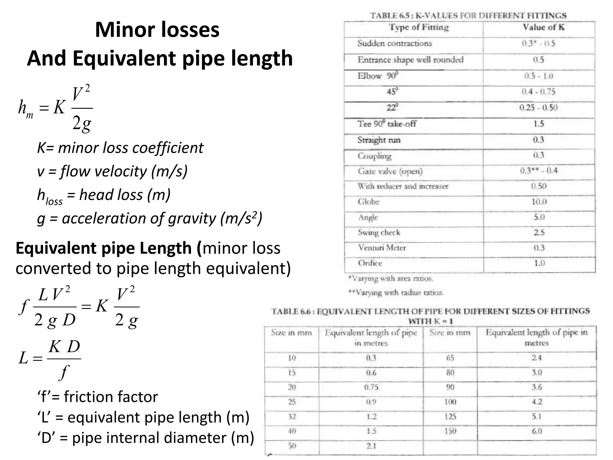
Head losses
Major Losses
Minor Losses
Definition • Dimensional Analysis • Types • Darcy Weisbech Equation • Major Losses • Minor Losses • Causes Head Losses
3. • Head loss is loss of energy per unit weight. • Head = Energy of Fluid / Weight • Head losses can be – Kinetic Head – Potential Head – Pressure Head 6/10/2015 4Danial Gondal Head Loss
4. • Kinetic Head – K.H. = kinetic energy / Weight = v² /2g • Potential Head – P.H = Potential Energy / Weight = mgz /mg = z • Pressure Head – P.H = P/ ρ g 6/10/2015 5
5. • (P/ ρ g) + (v² /2g ) + (z) = constant • (FL-2F-1L3LT-2L-1T2) + (L2T-2L1T2)+(L) = constant • (L) + (L) + (L) = constant • As L represent height so it is dimensionally L. 6/10/2015 6 Dimensional Analysis
6. • However the equation (P/ ρ g) + (v² /2g ) + (z) = constant Is valid for Bernoulli's Inviscid flow case. As we are studying viscous flow so (P1/ ρ g) + (v1² /2g ) + (z1) = EGL1(Energy Grade Line At point 1) (P2/ ρ g) + (v2² /2g ) + (z2) = EGL2(Energy Grade Line At point 2) 6/10/2015 7 Head Loss
7. • For Inviscid Flow EGL1 - EGL2= 0 • For Viscous Flow EGL1 - EGL2= Hf 6/10/2015 8 Head Loss
8. MAJOR LOSSES IN PIPES
9. •Friction loss is the loss of energy or “head” that occurs in pipe flow due to viscous effects generated by the surface of the pipe. • Friction Loss is considered as a "major loss" •In mechanical systems such as internal combustion engines, it refers to the power lost overcoming the friction between two moving surfaces. •This energy drop is dependent on the wall shear stress (τ) between the fluid and pipe surface. 6/10/2015 10 Friction Loss
10. •The shear stress of a flow is also dependent on whether the flow is turbulent or laminar. •For turbulent flow, the pressure drop is dependent on the roughness of the surface. •In laminar flow, the roughness effects of the wall are negligible because, in turbulent flow, a thin viscous layer is formed near the pipe surface that causes a loss in energy, while in laminar flow, this viscous layer is non-existent. 6/10/2015 11 Friction Loss
11. Frictional head losses are losses due to shear stress on the pipe walls. The general equation for head loss due to friction is the Darcy-Weisbach equation, which is where f = Darcy-Weisbach friction factor, L = length of pipe, D = pipe diameter, and V = cross sectional average flow velocity.
OPEN CHANNEL FLOW AND HYDRAULIC MACHINERY
Open channel flow: Types of flows – Type of channels – Velocity distribution – Energy and momentum correction factors – Chezy’s, Manning’s; and Bazin formula for uniform flow – Most Economical sections. Critical flow: Specific energy-critical depth – computation of critical depth – critical sub-critical – super critical flows
Non-uniform flows –Dynamic equation for G.V.F., Mild, Critical, Steep, horizontal and adverse slopes-surface profiles-direct step method- Rapidly varied flow, hydraulic jump, energy dissipation
Hardy cross method of pipe network analysissidrarashiddar
Hardy Cross Method of pipe network analysis has revolutionized the municipal water supply design. i.e., EPANET, a public domain software of water supply, uses the Hardy cross method for pipe network analysis. It is an iterative approach to estimate the flows within the pipe network where inflows (supply) and outflows (demand) with pipe characteristics are known.
Flow Equations for sluice gate.Introduces different flow equations to students which are widely utilized for the design of sluice gates connected to open channel.This tutorial will help to understand and articulate the basic flow equation utilized by designers all over the world.
Flow Through Pipes, Head Loss in Pipes, Minor Head Loss, Major Head Loss, Darcy's Formula, Chezy's Formula, Hydraulic Gradient Line, Total Energy Line, Energy Gradient Line... By Engr. M. Jalal Sarwar
Gradually varied flow is one kind of non uniform flow . Flow parameters such as depth of flow, flow velocity , discharge change with time and space gradually. Gradually varied flow is determined by the type of the channel bottom slopes. Flow profiles can be sustained in three different flow regions . This ppt covers only mild slope flow profile.
ntake structures are used for collecting water from the surface sources such as river, lake, and reservoir and conveying it further to the water treatment plant. These structures are masonry or concrete structures and provides relatively clean water, free from pollution, sand and objectionable floating material.
LARGE SCALE INSTALLATION OF SUBSURFACE DRAINAGE SYSTEM Tushar Dholakia
LARGE SCALE INSTALLATION OF SUBSURFACE DRAINAGE SYSTEM in Chambal Command, Rajasthan - Er. C.M. Tejawat, F.I.E., P. Eng., B.E. (Ag.), M.Sc. (Land Drainage Engineering) Deputy Director (Monitoring), CAD Chambal, Kota (Raj.)
The Role of Drainage Depth and Intensity on Hydrology and Nutrient Loss In th...LPE Learning Center
For more: http://www.extension.org/67691 Water management in the crop root-zone is crucial to successful crop growth and production. Irrigation, surface, and subsurface drainage—and other practices—are routinely implemented throughout the world to improve crop productivity and working conditions of the soil. Water management practices also impact the environmental footprint of agricultural systems by affecting the flow of water, nutrients, sediment, and other constituents through field, farms, and watersheds. Water management practices for agriculture in the Midwestern US should be designed with both profitability and the environment in mind. The design of subsurface (tile) drainage systems has traditionally been more a matter of how much drainage one can afford, rather than the aforementioned objectives. The relationship among subsurface drainage design characteristics (depth, spacing, layout), farm profitability, and environmental impact are not well known at the farm scale. Thus, drainage system design may fail to meet one or more of these important objectives. This presentation will examine the effects of subsurface drainage system design criteria on productivity, profitability, and the environment, using the soils and climatic conditions of the northern corn-belt (southern Minnesota). Water management in the crop root-zone is crucial to successful crop growth and production. Irrigation, surface, and subsurface drainage—and other practices—are routinely implemented throughout the world to improve crop productivity and working conditions of the soil. Water management practices also impact the environmental footprint of agricultural systems by affecting the flow of water, nutrients, sediment, and other constituents through field, farms, and watersheds. Water management practices for agriculture in the Midwestern US should be designed with both profitability and the environment in mind. The design of subsurface (tile) drainage systems has traditionally been more a matter of how much drainage one can afford, rather than the aforementioned objectives. The relationship among subsurface drainage design characteristics (depth, spacing, layout), farm profitability, and environmental impact are not well known at the farm scale. Thus, drainage system design may fail to meet one or more of these important objectives. This presentation will examine the effects of subsurface drainage system design criteria on productivity, profitability, and the environment, using the soils and climatic conditions of the northern corn-belt (southern Minnesota).
it speaks about the differential head flow meters. its different types. their principle of operation, venturi meter, orifice plate, rotameters, it also covers discussion on open channel flow meter. it covers the different application domains of the different types of flow meters and their advantages and disadvantages.
Energy losses in Bends, loss coefficient related to velocity head.Pelton Whee...Salman Jailani
In this slide you learn the how to make the lablayout and the study the Energy losses, Pelton Wheel. Kaplan TURBINE, Franices TURBine And its Efficiency of Mecahanical Power Plants..
00923006902338
Here you will get all information about sewer design, its type & various tests carried out on it for any leakage or any obstruction present and of improper joints.
deals with temperature, density, pressure, winds and humidity parameters of the atmosphere; Prssure gradient force, coriolis force, gravity force and friction force and winds and currents, ; pressure lows and highs, atmospheric circulation, winds.
Deals with the biological removal of nitrogen and phosphorus, Nitrification-denitrification removal of nitrogen, and Phosphate accumulating organisms and poly-hydroxibutirate in the phosphorus removal.
Artificial Reefs by Kuddle Life Foundation - May 2024punit537210
Situated in Pondicherry, India, Kuddle Life Foundation is a charitable, non-profit and non-governmental organization (NGO) dedicated to improving the living standards of coastal communities and simultaneously placing a strong emphasis on the protection of marine ecosystems.
One of the key areas we work in is Artificial Reefs. This presentation captures our journey so far and our learnings. We hope you get as excited about marine conservation and artificial reefs as we are.
Please visit our website: https://kuddlelife.org
Our Instagram channel:
@kuddlelifefoundation
Our Linkedin Page:
https://www.linkedin.com/company/kuddlelifefoundation/
and write to us if you have any questions:
info@kuddlelife.org
WRI’s brand new “Food Service Playbook for Promoting Sustainable Food Choices” gives food service operators the very latest strategies for creating dining environments that empower consumers to choose sustainable, plant-rich dishes. This research builds off our first guide for food service, now with industry experience and insights from nearly 350 academic trials.
Characterization and the Kinetics of drying at the drying oven and with micro...Open Access Research Paper
The objective of this work is to contribute to valorization de Nephelium lappaceum by the characterization of kinetics of drying of seeds of Nephelium lappaceum. The seeds were dehydrated until a constant mass respectively in a drying oven and a microwawe oven. The temperatures and the powers of drying are respectively: 50, 60 and 70°C and 140, 280 and 420 W. The results show that the curves of drying of seeds of Nephelium lappaceum do not present a phase of constant kinetics. The coefficients of diffusion vary between 2.09.10-8 to 2.98. 10-8m-2/s in the interval of 50°C at 70°C and between 4.83×10-07 at 9.04×10-07 m-8/s for the powers going of 140 W with 420 W the relation between Arrhenius and a value of energy of activation of 16.49 kJ. mol-1 expressed the effect of the temperature on effective diffusivity.
UNDERSTANDING WHAT GREEN WASHING IS!.pdfJulietMogola
Many companies today use green washing to lure the public into thinking they are conserving the environment but in real sense they are doing more harm. There have been such several cases from very big companies here in Kenya and also globally. This ranges from various sectors from manufacturing and goes to consumer products. Educating people on greenwashing will enable people to make better choices based on their analysis and not on what they see on marketing sites.
"Understanding the Carbon Cycle: Processes, Human Impacts, and Strategies for...MMariSelvam4
The carbon cycle is a critical component of Earth's environmental system, governing the movement and transformation of carbon through various reservoirs, including the atmosphere, oceans, soil, and living organisms. This complex cycle involves several key processes such as photosynthesis, respiration, decomposition, and carbon sequestration, each contributing to the regulation of carbon levels on the planet.
Human activities, particularly fossil fuel combustion and deforestation, have significantly altered the natural carbon cycle, leading to increased atmospheric carbon dioxide concentrations and driving climate change. Understanding the intricacies of the carbon cycle is essential for assessing the impacts of these changes and developing effective mitigation strategies.
By studying the carbon cycle, scientists can identify carbon sources and sinks, measure carbon fluxes, and predict future trends. This knowledge is crucial for crafting policies aimed at reducing carbon emissions, enhancing carbon storage, and promoting sustainable practices. The carbon cycle's interplay with climate systems, ecosystems, and human activities underscores its importance in maintaining a stable and healthy planet.
In-depth exploration of the carbon cycle reveals the delicate balance required to sustain life and the urgent need to address anthropogenic influences. Through research, education, and policy, we can work towards restoring equilibrium in the carbon cycle and ensuring a sustainable future for generations to come.
Prevalence of Toxoplasma gondii infection in domestic animals in District Ban...Open Access Research Paper
Toxoplasma gondii is an intracellular zoonotic protozoan parasite, infect both humans and animals population worldwide. It can also cause abortion and inborn disease in humans and livestock population. In the present study total of 313 domestic animals were screened for Toxoplasma gondii infection. Of which 45 cows, 55 buffalos, 68 goats, 60 sheep and 85 shaver chicken were tested. Among these 40 (88.88%) cows were negative and 05 (11.12%) were positive. Similarly 55 (92.72%) buffalos were negative and 04 (07.28%) were positive. In goats 68 (98.52%) were negative and 01 (01.48%) was recorded positive. In sheep and shaver chicken the infection were not recorded.
2. Pipeline/channel hydraulics
Head (m of water column – 0.102 m WC = 1.0 kPa)
• Total energy per unit weight of the flowing fluid (water)
• Includes 3 components
– Kinetic head (V2/2g)
– Potential head (Z)
– Pressure head (p/ρg)
HGL (Hydraulic Grade Line)
• Imaginary line corresponding to the sum of the potential head and
the pressure head drawn for a pipeline/channel
• For pipe flow it corresponds to the height to which water will rise
vertically in a tube attached to a pipeline
EGL (Energy Grade Line)
• Imaginary line corresponding to the sum of the velocity head, the
potential head and pressure head drawn for a pipeline/ channel
• EGL line is above HGL line at a vertical distance equivalent to the
velocity head of the flowing fluid
3. Pipeline/channel hydraulics
Head loss (hL)
• Frictional head loss (major losses)
– Water flow in a pipe/channel results in the development of
shear stress between the flowing water and the wetted wall and
result in head loss
– Depends on
• flow rate
• roughness of the surface
• length of the channel/pipe
• hydraulic radius
– Head loss due to friction (major losses) is calculated by
• Darcy-Weisbach formula and Hazen-Williams formula
• Mannings formula - Chezy formula
• Minor losses
– Turbulence due to appurtenances and fittings on the
pipelines/channels cause head loss
4. ρ = density (kg/m3)
dh = hydraulic diameter (m)
u = velocity (m/s)
μ = Dynamic viscosity (Ns/m2)
ν = Kinematic viscosity (m2/s)
hh
e
dudu
R
Reynolds Number
dh = hydraulic diameter (m)
A = area section of the duct (m2)
p = wetted perimeter of the duct (m)p
A
dh
4
Hydraulic diameter
g
V
d
L
fhf
2
2
f is coefficient of friction
L is length of pipe (m)
d is diameter of pipe (m)
V is mean velocity (m/s)
Darcy-Weisbach equation
5. f = D'Arcy-Weisbach friction coefficient
Re = Reynolds Number
k = roughness of duct/pipe/tube surface (m)
dh = hydraulic diameter (m)
fRd
k
f eh
51.2
72.3
log2
1
6.
7. 85.1
17.1
KC
V
R
L
hf hf is frictional head loss
V is velocity (m/s)
L is length of pipe (m)
R is hydraulic radius (m)
K is conversion factor (0.849 for SI units)
C is Hazen-William’s roughness coefficient
Q is flow rate (m3/sec.)
D is pipe diameter (m)
S is slope
Hazen-Williams equation
85.1
87.4
7.10
C
Q
D
L
hf
For circular pipe flow
54.063.2
54.063.0
2785.0
849.0
SDCQ
SRCV
‘C’ value increases with increasing internal smoothness, and increasing
pipe diameter, but decreases with pipe age
Plastic pipes have higher ‘C’ value (140) than iron pipes (130)
‘C’ value to a negligible extent is affected by changes in flow rates
For open channel flow
10. Equivalent pipe Length (minor loss
converted to pipe length equivalent)
g
V
Khm
2
2
K= minor loss coefficient
v = flow velocity (m/s)
hloss = head loss (m)
g = acceleration of gravity (m/s2)
f
DK
L
g
V
K
Dg
VL
f
22
22
‘f’= friction factor
‘L’ = equivalent pipe length (m)
‘D’ = pipe internal diameter (m)
Minor losses
And Equivalent pipe length
11. Pipes and pipe networks
Equivalent pipes
• A pipe is equivalent to another pipe when for a given head loss
same flow is produced
• Replacing a complex system of piping by a single equivalent pipe
Compound pipes
• pipes of several sizes in series
Branching pipes
• Two or more pipes branching out and not coming together again
downstream
Looping pipes
• Two or more pipes branching out and coming together downstream
(parallel pipes)
Pipe networks
• Flow analysis in pipe network for knowing flow rates – Hardy-Cross
method
12. Valves and gates for pipe flow
– Isolation or block valves; Flow control valves; Directional/Check
valves (non-return valves) and Pressure reducing valves
– Air release valves; Altitude valves and Float valves
Gates and sluice gates for open channel flow
Flow measurement devices for pipe flow
– Venturi meters and Orifice meters
– Current meters and Pitot tubes
– Electro-magnetic and sonic flow meters
Flow measurement devices for open channel flow
– V-notch, Rectangular weir, Proportional weir, Broad crested weirs
– Parshall flume, Venturi flume, and Palmer-Bolus flume
Pumps
– Centrifugal pumps; Reciprocating pumps; Open screw pumps
and Hydraulic ram pumps
Pumping stations
13. Best or most economic hydraulic cross
section for open channel flow
• Best or most economic hydraulic cross section for open channels
occur at the minimal wetted perimeter (or at the maximum
hydraulic radius) for a specific flow cross section
• For rectangular channels
widthdepthhas
channelgularrecfortioncrossfloweconomicmostandBest
giveszerotoderivativetheequating
y
yb
y
A
dy
dp
ytorespectwithderivativetaking
y
y
A
p
ybpperimeterwetted
byAtioncrossflow
2
1
tansec
2
.
2
2
2
.sec
22
14. Best or most economic hydraulic cross
section for open channel flow
For
..2 RP
D
y
21cos2 1
Ry
Ө is angle in radians
15. Scour velocity or Self cleansing velocity
• Self-cleansing velocity or scour velocity can be found by
Camp’s formula
• SG is specific gravity of the particle
• dp is particle size
• Ks is constant and its value is taken as 0.8
• Recommended self-cleansing velocity is 0.6 m/sec.
• Ensures transport of sand particles of 0.09 mm size and 2.65
specific gravity without allowing settling
• For preventing deposition of sand and gravel 0.75 m/sec.
velocity is recommended
• Velocity not exceeding 3.0 m/sec. is recommended for
avoiding damage channel damage from erosion
2
1
6
1
1
1
pS dSGKR
n
V
16. Water hammer
tCE
dk
C
g
VC
H
1
14250
.max
Hmax. Max. water hammer pressure (m)– occurs
when closure time is ≤ critical closure time
Increasing actual closure time decreases water
hammer pressure
C is velocity of the pressure wave/shock wave
(m/sec.)
High for rigid pipes- rigid pipes: 1370; steel
pipes: 850 and plastic pipes 200 m/sc.)
V0 is flow velocity prior to hammering (m/sec.)
‘k’ is bulk modulus of the water 2.07x10⁸ kg/m2
‘d’ is pipe diameter (m)
Ct is pipe wall thickness (m)
E is modulus of elasticity of pipe material
(kg/m2)
Modulus of elasticity
of pipe material
17. Water supply system may require valves sized up to 900mm dia.
normal range is 25 - 300mm dia.
Plumbing utilizes float valves in 15 - 100mm dia. Range.
Valves installed in applications outside their design limits give rise to problems such as
non shut-off, premature seat wear, high noise, water hammer or seat chatter
Selection, sizing and installation of the most appropriate float valve is very important
Design considerations include
•Providing high flow rates at low head loss (low running pressure at valve inlet)
•Designing the valve seat to minimize cavitation and noise
•Minimize valve’s internal frictional resistance
•Shut off loads whilst ensuring the float / lever mechanism is always in control
18.
19. Altitude and Level Control Valves
– These are employed at the point where pipeline enters a tank
– When tank level rises to a specified upper limit, the valve closes
to prevent any further flow eliminating overflow
– When the flow trend reverses, the valve reopens and allows the
tank to drain or to supply the usage demands of the system.
When valve inlet (system)
pressure falls below tank head
pressure, the altitude valve
opens to feed the system
When system pressure recovers
above tank head, the tank begins
to refill
When the high level set point is
reached, the valve will close
20. Air Release Valves
Used to release air trapped in pipelines (and to allow air into
empty pipelines under vacuum/negative gage pressure)
– Usually provided on both sides of an isolation valve, at the
system high points (summits), and at the points of pipeline
grade change (where negative pressures are possible)
Free air (air pockets) can be found in the pipelines (at high
points) and fittings
– Pressure change can cause release of dissolved air
– Air can enter pipelines by vortex action of pumps, at the intake
– Any openings, connections, and fittings can allow air to enter
What if air pockets are left in pipelines?
– Affect pipeline efficiency and intensify water hammering –
cause pressure surges and increase cavitation hazards
– Air in the water lines speeds up the corrosion process
– Air trapped at bends, tees and other fittings can reduce and
even stop flow
– Air can result in improper reading of customers’ meters
21. Air Release Valves
Valve Locations
• on rising mains after the pumps for both releasing and admitting air
• at high points throughout pipeline systems
• at pipeline slope transition points (before & after steep slopes)
• At every 500m distance on the long pipeline of uniform slope
Valve size: Air valve to conduit size is 1:12 for air release type
and 1:8 for air release as well as air admission
Valve operation
• Entry of the pipeline air into the valve body drops down the float
and allows the air to escape through the valve opening
• With the release of air, the pipeline water rises into the valve body
and lifts the float to its limit – pressing of the float against the seat
closes the valve opening and prevents the liquid escape
• When there is no flow in the pipeline, negative pressure developed
in the pipeline extends into the valve body and drops down the
float – this allows air entry through the valve into the pipeline
22.
23. Flow measurement
Rectangle Weirs:
• Contracted: Flow, Q = 3.33 (L - 0.2H) H1.5
• Suppressed: Flow, Q = 3.33 L(H1.5)
Q = Flow, cubic feet per second
L = Length of crest, feet
H = Upstream head, feet
Cipoletti Weirs: Flow, Q = 3.367 L(H1.5)
Q = Flow, cubic feet per second
L = Length of crest, feet
H = Upstream head, feet
V-Notch Weirs:
• 90' V-notch: Flow, Q = 2.50 H2.50
• 60' V-notch: Flow, Q = 1.443 H2.50
• 45' V-notch: Flow, Q = 1.035 H2.50
• 30' V-notch: Flow, Q = 0.685 H2.45
Q = Flow, cubic feet/second
H = Upstream head, feet
24. θ = v-notch angle
q = flow rate (m3/s)
h = head on the weir (m)
b = width of the weir (m)
g = 9.81 (m/s2) - gravity
cd= discharge constant for the weir - must be
determined
Rectangular Weir
q = 2/3 cd b (2 g)1/2 h3/2
Triangular or V-Notch Weir
q = 8/15 cd (2 g)1/2 tan(θ/2) h5/2
Broad-Crested Weir
q = cd h2 b ( 2 g (h1 - h2) )1/2
Common weir constructions are
rectangular weir (sharp-crested thin metal plate)
triangular or v-notch weir (sharp-crested thin metal plate)
broad-crested weir
trapezoidal (Cipolletti) weir
Sutro (proportional) weir
compound weirs (combination of the weirs of different shapes)
Weirs for flow measurement
25. Sluice gates for flow measurement
h = elevation height
ρ = density
v = flow velocity
According to Bernoulli Equation
1/2 ρ v1
2 + ρ g h1 = 1/2 ρ v2
2 + ρ g h2 -1
q = flow rate
A = flow area
b = width of the sluice
h1 = upstream height
h2 = downstream height
cd = discharge coefficient
ho = height sluice opening
According to the Continuity Equation:
q = v1 A1 = v2 A2 -2
q = v1 h1 b = v2 h2 b -3
1/2
12
2
1
12
21
2
1
1
2
21
2
]h[2 gv2
1
2
ghbhcq
hhfor
h
h
hhg
bhq
d
Combining equations -1 and -3
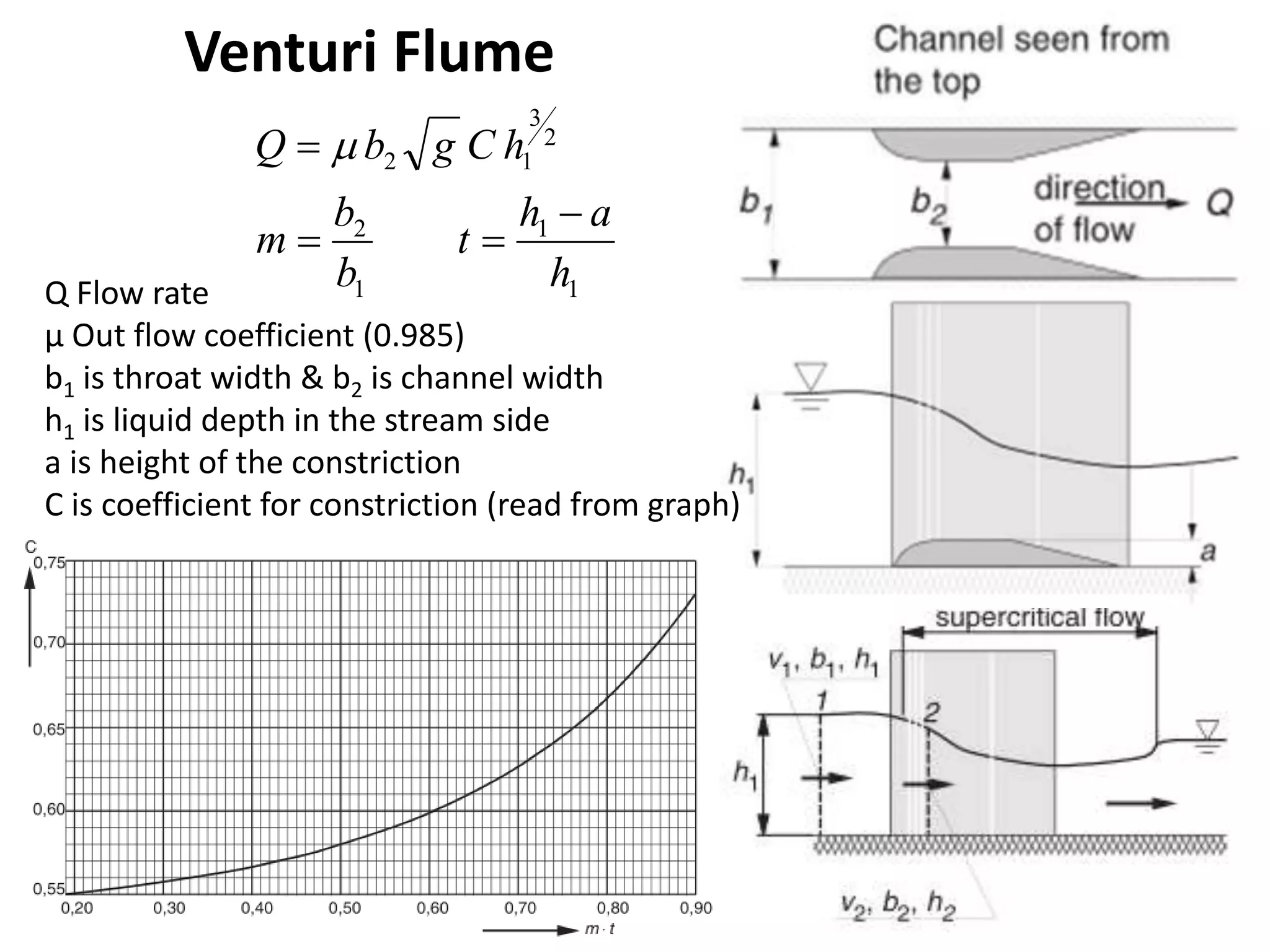
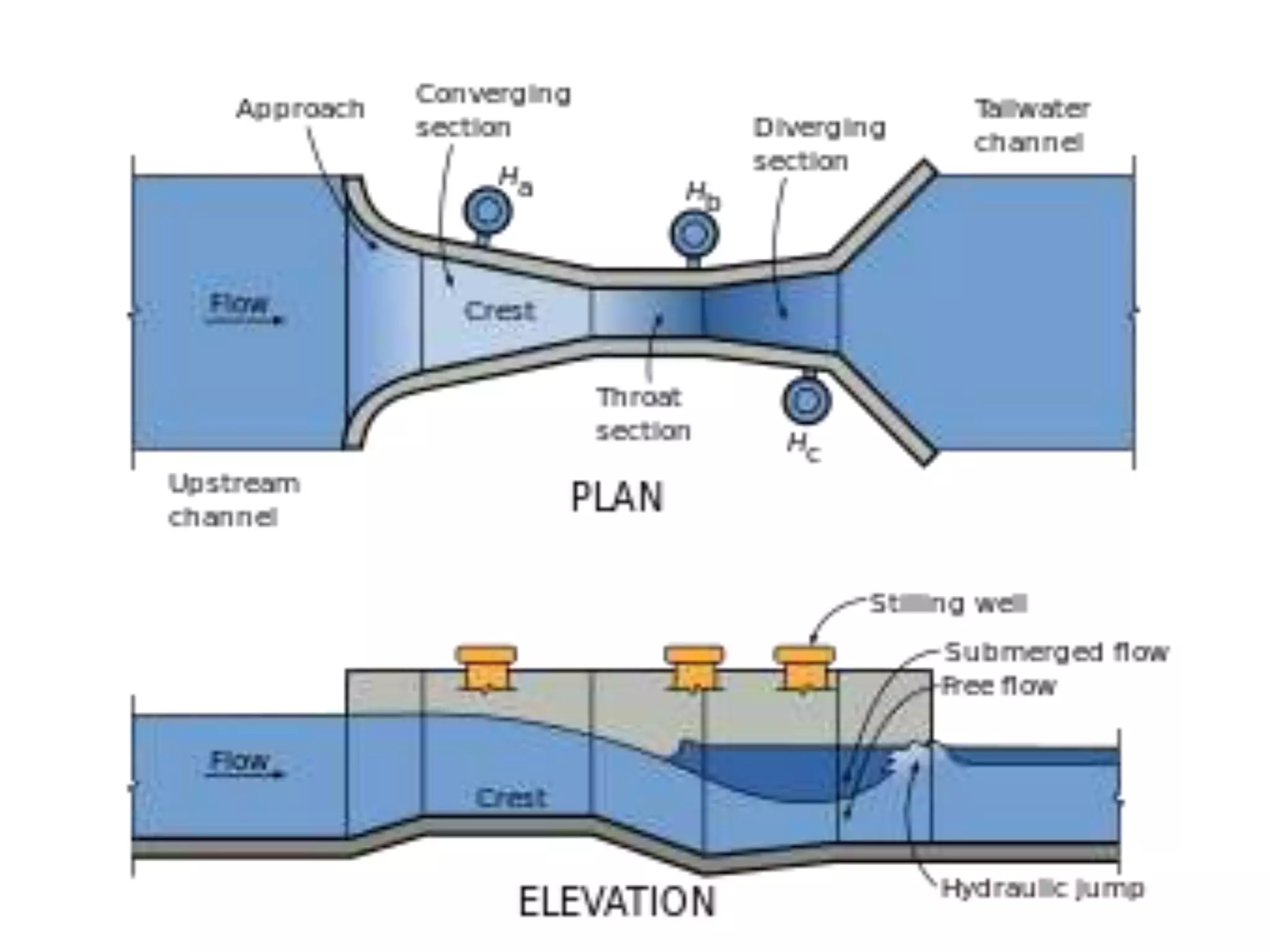
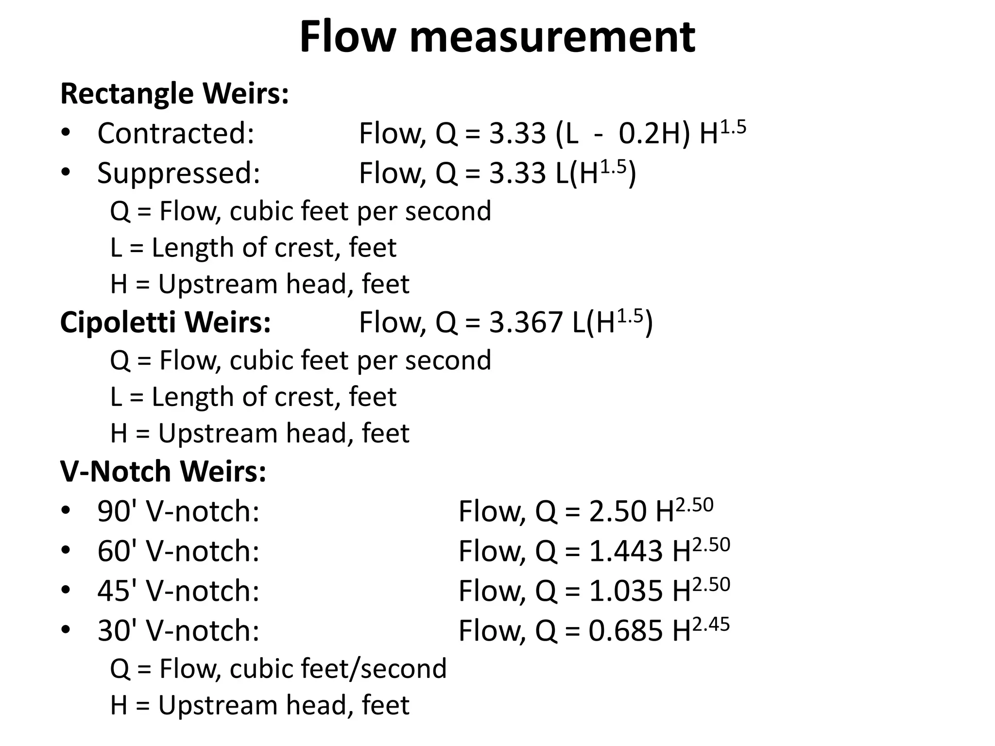
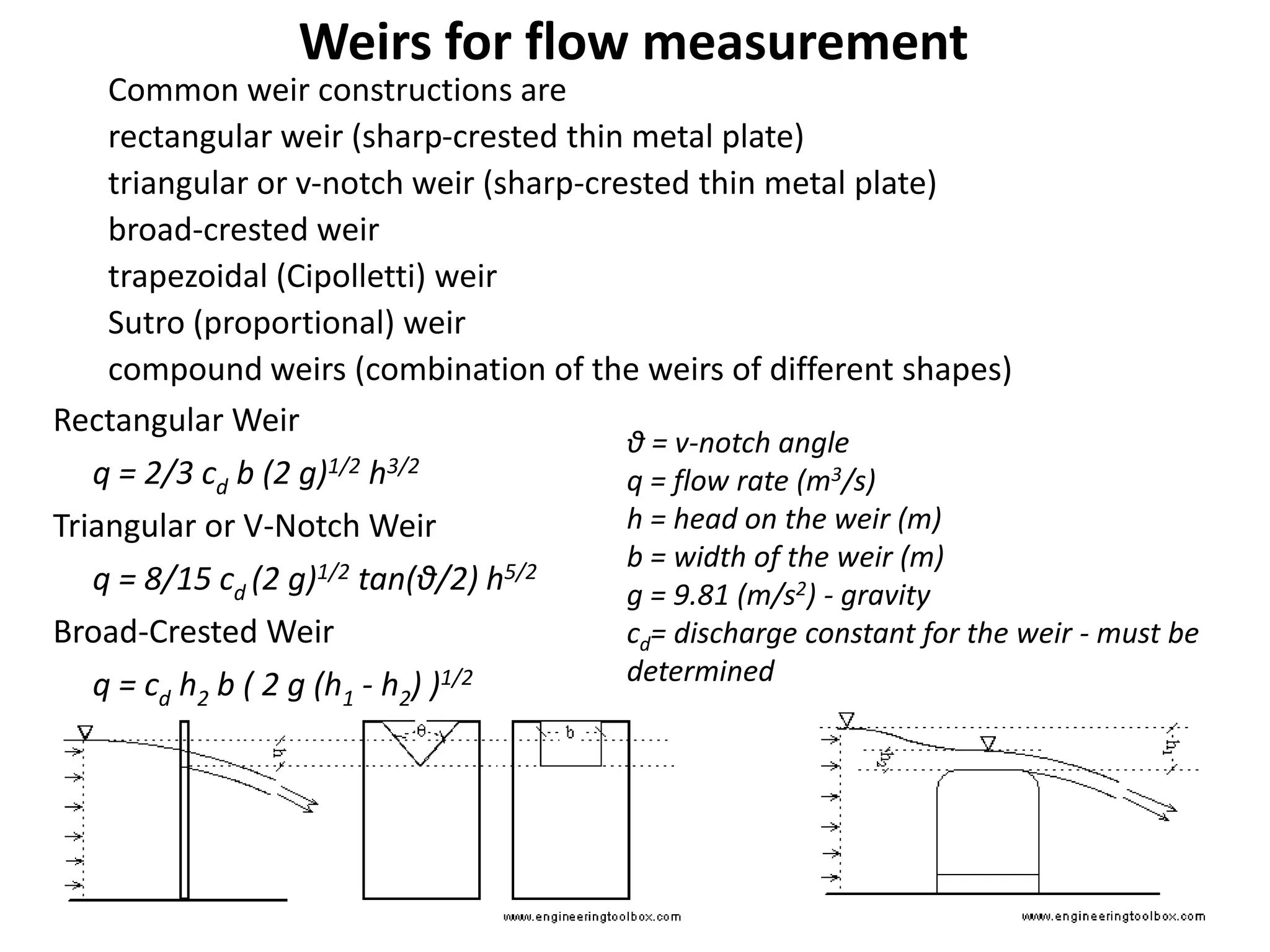
Used to measure flow rate in open channels
Pressures on the upstream and on the downstream are the same
cd is a function of opening height and vena
contracta height (cd = ho / h1 )
Its value is taken as ~ 0.61 for ho / h1 < 0.2
26. Q Flow rate
μ Out flow coefficient (0.985)
b1 is throat width & b2 is channel width
h1 is liquid depth in the stream side
a is height of the constriction
C is coefficient for constriction (read from graph)
Venturi Flume
1
1
1
2
2
3
12
h
ah
t
b
b
m
hCgbQ
27. Parshall Flume
A commonly used fixed hydraulic structure to measure flows in
channels
An improved venturi flume developed in 1915 by Ralph L. Parshall of
the U.S. Soil Conservation Service
A drop in elevation through the throat produced supercritical flow
through the throat of the flume and made only one head
measurement necessary to determine the flow rate
Parshall flume consists of a uniformly converging upstream section, a
short parallel throat section, and a uniformly diverging downstream
section
Floor of the flume is flat in the upstream section, slopes downward in
the throat, and then rises in the downstream section, ending with a
downstream elevation below that of the upstream elevation
Parshall flumes are constructed to the dimensions specified
22 sizes of Parshall flumes have been developed, covering flows from
0.1416 to 92,890 l/s (throat width, indicated as the flume size,
range from 1” to 50’)
28. Parshall Flume
Parshall flumes may operate under two conditions
• Free Flow condition: hydraulic jump is induced on the downstream
side and back water does not restrict flow through the flume –only
one depth (upstream) measurement is needed for flow calculation
• Submerged Flow condition: back water restricts flow through a
flume – for flow calculation depth measurement both upstream
and downstream is needed
When free-fall conditions exist for all flows, the throat and
downstream diverging sections of the flume may be left off
(Montana flume, a modified style of Parshall flume)
Parshall and Montana flume of the same throat width use the same
discharge tables and equations
When used in submerged flow applications, two head measurements,
one in the converging section and the other in the throat section,
are needed
Due to the added instrumentation costs and operational complexity of
operating under submerged flow conditions, operating flumes
under free-flow conditions is recommended
29. Q is flow rate
C is free-flow coefficient
Ha is head at the uptream
n varies with flume size
Free-flow discharge for the Parshall flume
Throat
Width
Coefficient
(C)
Exponent
(n)
1 in .338 1.55
2 in .676 1.55
3 in .992 1.55
6 in 2.06 1.58
9 in 3.07 1.53
1 ft 3.95 1.55
1.5 ft 6.00 1.54
2 ft 8.00 1.55
3 ft 12.00 1.57
4 ft 16.00 1.58
5 ft 20.00 1.59
6 ft 24.00 1.59
7 ft 28.00 1.60
8 ft 32.00 1.61
10 ft 39.38 1.60
12 ft 46.75 1.60
15 ft 57.81 1.60
20 ft 76.25 1.60
25 ft 94.69 1.60
30 ft 113.13 1.60
40 ft 150.00 1.60
50 ft 186.88 1.60
Flume Size St=Hb/Ha
1" - 3" 0.5
6" - 9" 0.6
1' - 8' 0.7
10' - 50' 0.8
For submerged flow
Hb/Ha is ≥ St - flow is submerged flow
Qnet = Q – Qcor.
Qcor. = M (0.000132 Ha
2.123 e9.284 (Hb/Ha))
M = multiplying factor
Q values are in ft3/s
Ha and Hb are in feet
Flume
Size
Factor,
M
1' 1
1.5' 1.4
2' 1.8
3' 2.4
4 3.1
5 3.7
6 4.3
7 4.9
8 5.4
Parshall Flume
35. Analysis of pump systems
Conducted to
– Select the most suitable pumping unit(s)
– Define operating point(s) of the pump(s)
Involves calculating the system head – capacity curves for the pumping
system and using these in conjunction with the head-capacity
curves of the available pumps
System head – capacity curve
– Graphical representation of the system head
– Developed by ploting total dynamic head over a range of flows from
zero to the maximum expected value
Pump head – capacity curve (pump characteristic curves)
– Illustrate relationship between head, capacity, efficiency and break
horse power over a wide range of possible operating conditions
Operating point:
– Plot pump head-capacity curve on the system head-capacity curve
– Intersection point of these two curves is operating point
36.
37.
38.
39. Pumping Stations
Components of a typical pumping station
• Wet well (sump)
• Dry well (pumping station!)
• Pumps and drives, piping with fittings (valves, gauges, etc.)
• Priming pumps, and seepage pump
• Electrical power control panels
• Crane or overhead girder
• Proper access to the pumps and drives
• Aisle space
• DG sets (for power backup!)
Pumping stations (types)
• Stations with only wet well (sump) and no dry well
– Using submersible (non-clog) pumps
– Using ground level (self-priming!) pumps (with a priming pump!)
• Stations with both wet well and dry well
– factory built dry well and non-clog pumps with top mounted drives
– Built on-site dry wells with pumps installed at the bottom