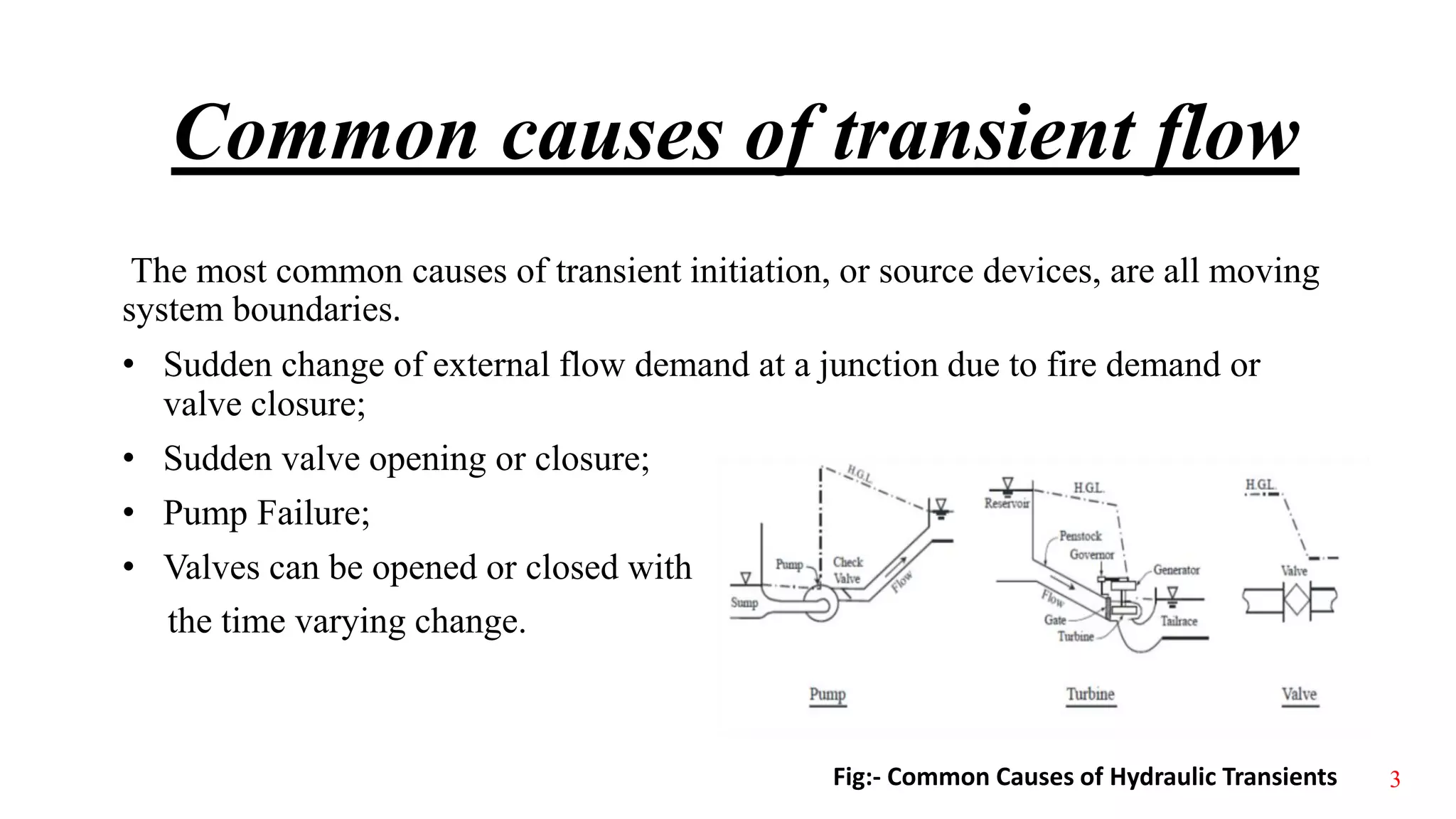
SlideShare a Scribd company logo
MODELING OF TRANSIENT FLUID
FLOW IN THE SIMPLE PIPELINE
SYSTEM
Submitted by:-
Aniruddha Singha (184104602)
What is Transient Flow
 A transient is a temporary flow and pressure condition that occurs in a hydraulic system
between an initial steady-state condition and a final steady-state condition;
 When velocity changes rapidly in response to the operation of a flow-control device(for
instance, a valve closure or pump start), the compressibility of the liquid and the elasticity of
the pipeline cause a transient pressure wave to propagate throughout the system;
 In general, transients resulting from relatively slow changes in flow rate are referred to as
surges, and those resulting from more rapid changes in flow rate are referred to as water
hammer events. Surges in pressurized systems are different than tidal or storm
surges, flood waves, or dam breaks, which can occur in open-water bodies;
 In general engineering practice, the terms surge, transient and water hammer are synonymous.
1
Methods for Formulation of transient flow
• Various methods have been developed to solve transient flow in pipes. These range from approximate equations to
numerical solutions of the nonlinear Navier-Stokes equations:
I. Arithmetic method—Assumes that flow stops instantaneously (in less than the characteristic time, 2L/a),
cannot handle water column separation directly, and neglects friction (Joukowski, 1898; Allievi, 1902).
II. Graphical method—Neglects friction in its theoretical development but includes a means of accounting for it
through a correction (Parmakian, 1963). It is time consuming and not suited to solving networks or pipelines with
complex profiles.
III. Method of Characteristics (MOC)—Most widely used and tested approach, with support for complex boundary
conditions and friction and vaporous cavitation models. It converts the partial differential equations(PDEs) of
continuity and momentum (e.g., Navier-Stokes) into ordinary differential equations that are solved algebraically
along lines called characteristics.
2
Common causes of transient flow
The most common causes of transient initiation, or source devices, are all moving
system boundaries.
• Sudden change of external flow demand at a junction due to fire demand or
valve closure;
• Sudden valve opening or closure;
• Pump Failure;
• Valves can be opened or closed with
the time varying change.
Fig:- Common Causes of Hydraulic Transients 3
Valves : A valve can start, change, or stop flow very suddenly. Energy
conservations increase or decrease in proportion to a valve’s closing or opening
rate and position , or stroke . Orifices can be used to throttle flow instead of a
partially open valve . Valves can also allow air into a pipeline and/or expel it,
typically at local high points.
(The problem that has been formulated for transient flow in pipelines is
due to closure of valve).
In pressurized networks, a steady-state condition or transient event at one
point in the system can affect all other parts of the system. Consequently,
computer models must consider every pipe that is directly connected to a
pressurized system, regardless of administrative or political boundaries.
4
Wave Propagation
The sequence of events following valve closure may be divided into four parts (Fig) as follows:
1. 0 < t ≤ L/a
When the valve is closed the flow velocity at the valve becomes zero. This increases the pressure at the valve by ΔH = -(a/g) ΔV.
and a positive pressure wave propagates towards the reservoir at the upstream. If a is the velocity of the pressure wave and L is
the length of the pipeline, then the wave front reaches the upstream reservoir at time t = L/a. At this time, along the entire length
of the pipeline, the pipe is expanded, the flow velocity is zero, and the pressure head is Ho + ΔH .
2. L/a < t ≤ 2L/a
Just as the wave reaches the upstream reservoir, pressure at a section on the reservoir side is Ho while the pressure at an adjacent
section in the pipe is Ho + ΔH. Because of this difference in pressure, the fluid flows from the pipeline into the reservoir with
velocity -Vo. Thus, the flow velocity at the pipe entrance is reduced from zero to -Vo.
3. 2L/a < t ≤ 3L/a
Since the valve is completely closed, a negative velocity cannot be maintained at the valve. Therefore, the velocity changes
instantaneously from −Vo to 0, the pressure drops to Ho − ΔH, and a negative wave propagates towards the reservoir
Behind this wave front, the pressure is Ho - ΔH and the fluid velocity is zero. The wave front reaches the upstream reservoir
at time t = 3L/a, the pressure head in the entire pipeline is Ho - ΔH, and the fluid velocity is zero.
.
5
4. 3L/a < t ≤ 4L/a
As soon as this negative wave reaches the reservoir, an unbalanced condition is created again at the
upstream end. Now the pressure is higher on the reservoir side than at an adjacent section in the
pipeline. Therefore, the fluid now flows from the reservoir into the pipeline with velocity Vo, and the
pressure head increases to Ho .At time t = 4L/a the wave front reaches the downstream valve, the
pressure head in the entire pipeline is Ho, and the flow velocity is Vo. Thus, the conditions in the pipeline
at this time are the same as those during the initial steady-state conditions except that the valve is now
closed.
Since the valve is completely closed, the preceding sequence of events starts again at t = 4L/a
Fig:- Pressure variation at valve
6
Formulation of problem
During the hydraulic shock (water hammer) in the metal pipe, the
velocity c of the pressure disturbance is usually three times greater than
the velocity v of the flow, which therefore, may be ignored in the
characteristic equations
𝑑𝑥
𝑑𝑡
= ± c (1)
In the simplified analysis, fluid viscosity is neglected, which means that
in the equation:
±
𝑔
𝑐
𝑑ℎ
𝑑𝑡
+
𝑑𝑣
𝑑𝑡
+
λ𝑣∣𝑑𝑣∣
2𝑑
= 0 (2)
7
The last member is cancelled, i.e.
λ𝑣∣𝑑𝑣∣
2𝑑
= 0 . Considering the reductions mentioned, simple pipeline system is
analysed as shown in Figures below
Fig:- Diagram x-t for the basic version
of the simple pipeline Fig:- Schematic diagram of pipe system
8
1. Continuity Equation for Unsteady Flow
The continuity equation for a fluid is based on the principle of conservation of mass.
The general form of the continuity equation for unsteady fluid flow is as follows :
𝑎2 𝜕𝑄
𝜕𝑥
+ 𝑔𝐴
𝜕𝐻
𝜕𝑡
=0
2. Momentum Equation for Unsteady Flow
The equations of motion for a fluid can be derived from the consideration of the forces
acting on a small element, or control volume, including the shear stresses generated by
the fluid motion and viscosity. The three-dimensional momentum equations of a real
fluid system are known as the Navier-Stokes equations. Since flow perpendicular to
pipe walls is approximately zero, flow in a pipe can be considered one-dimensional, for
which the continuity equation reduces to
𝜕𝑄
𝜕𝑡
+ 𝑔𝐴
𝜕𝐻
𝜕𝑥
+R𝑄 ∣ 𝑄 ∣= 0
9
Data used for the problem
• The height of the water pressure in the tank, h = 100m
• The length of the pipe, l = 12000 m
• Number of pipes in the system, n = 4
• Pipe diameter, D = 900mm
• Pressure wave velocity, c = 1200 m/s
• Coefficient of friction resistance, f= 0.022
• Δx=l/n=3000 m
• Δt=6 sec
Initial values
ℎ1=100 at t=0,6,12………
ℎ2= 99.83 at t=0
10
ℎ3=99.50 at t=0
ℎ4= 98.70 at t=0
ℎ5=98.5 at t=0
Known values of discharge taken
Q(:,1)=2.63; Q(1,2)=1.89; Q(1,3)=0.6; Q(1,4)=0.2
11
Lax Scheme
The numerical scheme used in the problem is the Lax Scheme. This scheme is first-
order accurate, is easy to program and gives satisfactory results although sharp wave
fronts are slightly smeared.
The partial derivatives as follows:-
𝜕𝐻
𝜕𝑡
=
𝐻𝑖
𝑗+1
− 𝐻𝑖
Δ𝑡
𝜕𝑄
𝜕𝑡
=
𝑄𝑖
𝑗+1
− 𝑄𝑖
Δ𝑡
𝜕𝑄
𝜕𝑥
=
𝑄𝑖+1
𝑗
− 𝑄𝑖−1
𝑗
2Δ𝑥
𝜕𝐻
𝜕𝑥
=
𝐻𝑗+1
𝑖
− 𝐻𝑖−1
𝑗
2Δ𝑥 12
In which
ഥ𝐻𝑖 = 0.5(𝐻𝑗+1
𝑖
− 𝐻𝑖−1
𝑗
) and
ത𝑄𝑖 = 0.5(𝑄𝑗+1
𝑖
− 𝑄𝑖−1
𝑗
)
Putting the above equations in Continuity and momentum equation we have,
𝐻𝑖
𝑗+1
=0.5(𝐻𝑖−1
𝑗
+𝐻𝑖+1
𝑗
)-0.5
𝑎2
𝑔𝐴
Δ𝑡
Δ𝑥
(𝑄𝑖+1
𝑗
− 𝑄𝑖−1
𝑗
)
and
𝑄𝑖
𝑗+1
=0.5(𝑄𝑖−1
𝑗
+𝑄𝑖+1
𝑗
)-0.5𝑔𝐴
Δ𝑡
Δ𝑥
(𝐻𝑖+1
𝑗
− 𝐻𝑖−1
𝑗
) − RΔ𝑡 ത𝑄𝑖| ത𝑄𝑖|
Fig:- Elementary mesh of
characteristics grid for internal
points
13
MATLAB Code
h = 100 ; %The height of the water pressure in the tank,m
l = 12000 ; %The length of the pipe,m
n = 4 ; % Number of pipes in the system,
D = 900/1000; %Pipe diameter, Pipe diameter,mm
c = 1200 ; % velocity of pressure wave,m/s
f= 0.022 ; % Coefficient of friction resistance,
g=9.8 ; %acceleration due to gravity,m/s^2
Q=2.63; %discharge in first node,m^3/s
A=(pi*D^2)/4; %Area of pipe,m^2
V=Q/A; %velocity of water,m/s
%hf=(f*l/n*V^2)/(2*g*D); %%head loss in second node by weisbach equation
hf=.345;
H=100; %head in first node
15
h1=99.83; h2=99.50; h3=98.7; h4=98.5; %%% head in each node,m
R=f/(2*D*A^2);
deltax=l/n; %dx
deltat=6; %dt
hh=zeros(8,5);
hh(:,1)=100; hh(1,2)=h1; hh(1,3)=h2; hh(1,4)=h3;
hh(1,5)=h4; %%head loss matrix
qq=zeros(8,5);
qq(:,1)=2.63; qq(1,2)=1.89; qq(1,3)=.6; qq(1,4)=.2;
qq(1,5)=.39; %%discharge matrix
t=0:6:42;
for i=1:7
for j=1:3
hh(i+1,j+1)=hh(i,j)+hh(i,j+2)-(c^2/(2*g*A))*(deltat/deltax)*(qq(i,j)-qq(i,j+2));
for k=1:8
q(k,j+1)=1/2*(qq(k,j)+qq(k,j+2))
end
qq(i+1,j+1)=1/2*(qq(i,j)+qq(i,j+2))-(g*A/2)*(deltat/deltax)*(hh(i,j)-hh(i,j+2))-R *q(i,j+1)*abs(q(i,j+1))*deltat
end
16
end
n=3; %node number
subplot(2,1,1);
plot(t',hh(:,n),'g')
xlabel('time(sec)','Fontsize',12);
ylabel('head (m)','Fontsize',12)
subplot(2,1,2);
plot(t',qq(:,n),'r')
xlabel('time(sec)','Fontsize',12);
ylabel('discharge(cumec)','Fontsize',12)
17
Output
For node 1
18
For node 2
19
For node 3
20
For node 4
21
For node 5
22
Conclusion
 The construction of reliable and efficient piping systems represents a large
investment cost due to the number of protective elements to be installed to keep the
system safe from non-stationary phenomena;
 The terms for one-dimensional fluid flow, with the introduction of assumptions and
simplifications, are quite complex, therefore MATLAB programs is used to calculate
fluid flow parameters;
 In the numerical calculations advantage has been taken of the Lax Scheme which
can be used in the cases when frictional effects are very important. In this method
the values of the pressure heads and discharge flows are calculated on the basis of
the mean resistance of elementary pipe sections related to the flow value of the
preceding and following time steps.
14
References
 Salmanzadeh M. (1993) “Numerical Method for Modeling Transient Flow in
Distribution Systems”, Islamic Azad University, Shoushtar;
 Vataj G. & Berisha X. (2018) “MODELING OF TRANSIENT FLUID FLOW IN
THE SIMPLE PIPELINE SYSTEM”, University of Prishtina, Pristina, Kosovo;
 Textbook of APPLIED HYDRAULIC TRANSIENTS by M. Hanif Chaudhry.
23
Modeling of transient fluid flow in the simple pipeline system

More Related Content

What's hot

Desin of penstock pipe ppt
Desin of penstock pipe pptDesin of penstock pipe ppt
Desin of penstock pipe ppt
zafaralam7868
 
Flow through pipes ppt
Flow through pipes pptFlow through pipes ppt
Flow through pipes ppt
Vishal Chaudhari
 
ORIFICES AND MOUTHPIECES
ORIFICES AND MOUTHPIECESORIFICES AND MOUTHPIECES
ORIFICES AND MOUTHPIECES
Home
 
Fluid kinematics
Fluid kinematicsFluid kinematics
Fluid kinematics
Mohsin Siddique
 
Centrifugal Pumps
Centrifugal PumpsCentrifugal Pumps
Centrifugal Pumps
Malla Reddy University
 
PRESSURE & HEAD (PART-1)
PRESSURE & HEAD (PART-1)PRESSURE & HEAD (PART-1)
PRESSURE & HEAD (PART-1)
KHORASIYA DEVANSU
 
Open channel flow equation
Open channel flow equationOpen channel flow equation
Open channel flow equation
Mrinmoy Majumder
 
Types of flow in open channel
Types of flow in open channelTypes of flow in open channel
Types of flow in open channel
Mir Zafarullah
 
Head losses
Head lossesHead losses
Head losses
Faizan Shabbir
 
Open channels
Open channelsOpen channels
Open channels
Samer Elabd
 
Energy quations and its application
Energy quations and its applicationEnergy quations and its application
Energy quations and its application
Sagar Damani
 
open channel flow
open channel flowopen channel flow
open channel flow
GeoRuizO
 
Fluid Mechanics - Fluid Pressure and its measurement
Fluid Mechanics - Fluid Pressure and its measurementFluid Mechanics - Fluid Pressure and its measurement
Fluid Mechanics - Fluid Pressure and its measurement
Malla Reddy University
 
Boundary layer
Boundary layerBoundary layer
Boundary layer
Vishal Chaudhari
 
UNIT 1 UNIFORM FLOW.pptx
UNIT 1 UNIFORM FLOW.pptxUNIT 1 UNIFORM FLOW.pptx
UNIT 1 UNIFORM FLOW.pptx
reenarana28
 
laminar and Turbulent flow
laminar and Turbulent flowlaminar and Turbulent flow
laminar and Turbulent flow
Vikramsinh Tiware
 
Fluid Kinematics
Fluid KinematicsFluid Kinematics
Fluid Kinematics
Malla Reddy University
 
Pumps
PumpsPumps

What's hot (20)

Orifice and mouthpieces
Orifice and mouthpieces Orifice and mouthpieces
Orifice and mouthpieces
 
Desin of penstock pipe ppt
Desin of penstock pipe pptDesin of penstock pipe ppt
Desin of penstock pipe ppt
 
Flow through pipes ppt
Flow through pipes pptFlow through pipes ppt
Flow through pipes ppt
 
ORIFICES AND MOUTHPIECES
ORIFICES AND MOUTHPIECESORIFICES AND MOUTHPIECES
ORIFICES AND MOUTHPIECES
 
Fluid kinematics
Fluid kinematicsFluid kinematics
Fluid kinematics
 
Centrifugal Pumps
Centrifugal PumpsCentrifugal Pumps
Centrifugal Pumps
 
PRESSURE & HEAD (PART-1)
PRESSURE & HEAD (PART-1)PRESSURE & HEAD (PART-1)
PRESSURE & HEAD (PART-1)
 
Open channel flow equation
Open channel flow equationOpen channel flow equation
Open channel flow equation
 
Types of flow in open channel
Types of flow in open channelTypes of flow in open channel
Types of flow in open channel
 
Bl concept
Bl conceptBl concept
Bl concept
 
Head losses
Head lossesHead losses
Head losses
 
Open channels
Open channelsOpen channels
Open channels
 
Energy quations and its application
Energy quations and its applicationEnergy quations and its application
Energy quations and its application
 
open channel flow
open channel flowopen channel flow
open channel flow
 
Fluid Mechanics - Fluid Pressure and its measurement
Fluid Mechanics - Fluid Pressure and its measurementFluid Mechanics - Fluid Pressure and its measurement
Fluid Mechanics - Fluid Pressure and its measurement
 
Boundary layer
Boundary layerBoundary layer
Boundary layer
 
UNIT 1 UNIFORM FLOW.pptx
UNIT 1 UNIFORM FLOW.pptxUNIT 1 UNIFORM FLOW.pptx
UNIT 1 UNIFORM FLOW.pptx
 
laminar and Turbulent flow
laminar and Turbulent flowlaminar and Turbulent flow
laminar and Turbulent flow
 
Fluid Kinematics
Fluid KinematicsFluid Kinematics
Fluid Kinematics
 
Pumps
PumpsPumps
Pumps
 

Similar to Modeling of transient fluid flow in the simple pipeline system

CH7 PC and SR.pptx
CH7 PC and SR.pptxCH7 PC and SR.pptx
CH7 PC and SR.pptx
Dawit Girma
 
Hidráulica
Hidráulica Hidráulica
Hidráulica
MarielaAguilera11
 
Basic equation of fluid flow mechan.pptx
Basic equation of fluid flow mechan.pptxBasic equation of fluid flow mechan.pptx
Basic equation of fluid flow mechan.pptx
AjithPArun1
 
FYP Presentation v2.0
FYP Presentation v2.0FYP Presentation v2.0
FYP Presentation v2.0Bianchi Dy
 
Flow of incompressible fluids through pipes
Flow of incompressible fluids through pipes Flow of incompressible fluids through pipes
Flow of incompressible fluids through pipes
MAULIKM1
 
Piping Design_Unit 1.pptx
Piping Design_Unit 1.pptxPiping Design_Unit 1.pptx
Piping Design_Unit 1.pptx
Abhay Rajput
 
Ch.1 fluid dynamic
Ch.1 fluid dynamicCh.1 fluid dynamic
Ch.1 fluid dynamic
Malika khalil
 
Fluid Flow inside and outside of the pipe
Fluid Flow inside and outside of the pipeFluid Flow inside and outside of the pipe
Fluid Flow inside and outside of the pipe
Amin394100
 
FLUID-MECHANICS-AND-MASS-TRANSFAR-FM7.pdf
FLUID-MECHANICS-AND-MASS-TRANSFAR-FM7.pdfFLUID-MECHANICS-AND-MASS-TRANSFAR-FM7.pdf
FLUID-MECHANICS-AND-MASS-TRANSFAR-FM7.pdf
rohitkumar00486
 
9-Viscous flow in ducts.pptx
9-Viscous flow in ducts.pptx9-Viscous flow in ducts.pptx
9-Viscous flow in ducts.pptx
Daniel678511
 
007c (PPT) Pitot tube, Notches & Weirs.pdf
007c (PPT) Pitot tube, Notches & Weirs.pdf007c (PPT) Pitot tube, Notches & Weirs.pdf
007c (PPT) Pitot tube, Notches & Weirs.pdf
happycocoman
 
CHAPTER_4C-Water-Hammer.ppt
CHAPTER_4C-Water-Hammer.pptCHAPTER_4C-Water-Hammer.ppt
CHAPTER_4C-Water-Hammer.ppt
SomayehSarabadan
 
Flow through Pipes .pptx
Flow through Pipes .pptxFlow through Pipes .pptx
Flow through Pipes .pptx
jadhavrushi403
 
Flow through pipes
Flow through pipesFlow through pipes
Flow through pipes
vaibhav tailor
 
pipe friction for laminar
pipe friction for laminarpipe friction for laminar
pipe friction for laminar
Muhammed Fuad Al-Barznji
 
0 open channel intro 5
0 open channel   intro 50 open channel   intro 5
0 open channel intro 5
Refee Lubong
 
pipe friction for laminar
pipe friction for laminarpipe friction for laminar
pipe friction for laminar
Muhammed Fuad Al-Barznji
 
Diapositivas ecuación de continuidad
Diapositivas ecuación de continuidadDiapositivas ecuación de continuidad
Diapositivas ecuación de continuidad
ErikCalvopia
 
Ecuación de continuidad
Ecuación de continuidad Ecuación de continuidad
Ecuación de continuidad
ErikCalvopia
 
0exp11 pipe friction_01
0exp11 pipe friction_010exp11 pipe friction_01
0exp11 pipe friction_01
Muhammed Fuad Al-Barznji
 

Similar to Modeling of transient fluid flow in the simple pipeline system (20)

CH7 PC and SR.pptx
CH7 PC and SR.pptxCH7 PC and SR.pptx
CH7 PC and SR.pptx
 
Hidráulica
Hidráulica Hidráulica
Hidráulica
 
Basic equation of fluid flow mechan.pptx
Basic equation of fluid flow mechan.pptxBasic equation of fluid flow mechan.pptx
Basic equation of fluid flow mechan.pptx
 
FYP Presentation v2.0
FYP Presentation v2.0FYP Presentation v2.0
FYP Presentation v2.0
 
Flow of incompressible fluids through pipes
Flow of incompressible fluids through pipes Flow of incompressible fluids through pipes
Flow of incompressible fluids through pipes
 
Piping Design_Unit 1.pptx
Piping Design_Unit 1.pptxPiping Design_Unit 1.pptx
Piping Design_Unit 1.pptx
 
Ch.1 fluid dynamic
Ch.1 fluid dynamicCh.1 fluid dynamic
Ch.1 fluid dynamic
 
Fluid Flow inside and outside of the pipe
Fluid Flow inside and outside of the pipeFluid Flow inside and outside of the pipe
Fluid Flow inside and outside of the pipe
 
FLUID-MECHANICS-AND-MASS-TRANSFAR-FM7.pdf
FLUID-MECHANICS-AND-MASS-TRANSFAR-FM7.pdfFLUID-MECHANICS-AND-MASS-TRANSFAR-FM7.pdf
FLUID-MECHANICS-AND-MASS-TRANSFAR-FM7.pdf
 
9-Viscous flow in ducts.pptx
9-Viscous flow in ducts.pptx9-Viscous flow in ducts.pptx
9-Viscous flow in ducts.pptx
 
007c (PPT) Pitot tube, Notches & Weirs.pdf
007c (PPT) Pitot tube, Notches & Weirs.pdf007c (PPT) Pitot tube, Notches & Weirs.pdf
007c (PPT) Pitot tube, Notches & Weirs.pdf
 
CHAPTER_4C-Water-Hammer.ppt
CHAPTER_4C-Water-Hammer.pptCHAPTER_4C-Water-Hammer.ppt
CHAPTER_4C-Water-Hammer.ppt
 
Flow through Pipes .pptx
Flow through Pipes .pptxFlow through Pipes .pptx
Flow through Pipes .pptx
 
Flow through pipes
Flow through pipesFlow through pipes
Flow through pipes
 
pipe friction for laminar
pipe friction for laminarpipe friction for laminar
pipe friction for laminar
 
0 open channel intro 5
0 open channel   intro 50 open channel   intro 5
0 open channel intro 5
 
pipe friction for laminar
pipe friction for laminarpipe friction for laminar
pipe friction for laminar
 
Diapositivas ecuación de continuidad
Diapositivas ecuación de continuidadDiapositivas ecuación de continuidad
Diapositivas ecuación de continuidad
 
Ecuación de continuidad
Ecuación de continuidad Ecuación de continuidad
Ecuación de continuidad
 
0exp11 pipe friction_01
0exp11 pipe friction_010exp11 pipe friction_01
0exp11 pipe friction_01
 

Recently uploaded

basic-wireline-operations-course-mahmoud-f-radwan.pdf
basic-wireline-operations-course-mahmoud-f-radwan.pdfbasic-wireline-operations-course-mahmoud-f-radwan.pdf
basic-wireline-operations-course-mahmoud-f-radwan.pdf
NidhalKahouli2
 
Unbalanced Three Phase Systems and circuits.pptx
Unbalanced Three Phase Systems and circuits.pptxUnbalanced Three Phase Systems and circuits.pptx
Unbalanced Three Phase Systems and circuits.pptx
ChristineTorrepenida1
 
Heap Sort (SS).ppt FOR ENGINEERING GRADUATES, BCA, MCA, MTECH, BSC STUDENTS
Heap Sort (SS).ppt FOR ENGINEERING GRADUATES, BCA, MCA, MTECH, BSC STUDENTSHeap Sort (SS).ppt FOR ENGINEERING GRADUATES, BCA, MCA, MTECH, BSC STUDENTS
Heap Sort (SS).ppt FOR ENGINEERING GRADUATES, BCA, MCA, MTECH, BSC STUDENTS
Soumen Santra
 
Final project report on grocery store management system..pdf
Final project report on grocery store management system..pdfFinal project report on grocery store management system..pdf
Final project report on grocery store management system..pdf
Kamal Acharya
 
Modelagem de um CSTR com reação endotermica.pdf
Modelagem de um CSTR com reação endotermica.pdfModelagem de um CSTR com reação endotermica.pdf
Modelagem de um CSTR com reação endotermica.pdf
camseq
 
DESIGN AND ANALYSIS OF A CAR SHOWROOM USING E TABS
DESIGN AND ANALYSIS OF A CAR SHOWROOM USING E TABSDESIGN AND ANALYSIS OF A CAR SHOWROOM USING E TABS
DESIGN AND ANALYSIS OF A CAR SHOWROOM USING E TABS
itech2017
 
Nuclear Power Economics and Structuring 2024
Nuclear Power Economics and Structuring 2024Nuclear Power Economics and Structuring 2024
Nuclear Power Economics and Structuring 2024
Massimo Talia
 
MCQ Soil mechanics questions (Soil shear strength).pdf
MCQ Soil mechanics questions (Soil shear strength).pdfMCQ Soil mechanics questions (Soil shear strength).pdf
MCQ Soil mechanics questions (Soil shear strength).pdf
Osamah Alsalih
 
Recycled Concrete Aggregate in Construction Part III
Recycled Concrete Aggregate in Construction Part IIIRecycled Concrete Aggregate in Construction Part III
Recycled Concrete Aggregate in Construction Part III
Aditya Rajan Patra
 
RAT: Retrieval Augmented Thoughts Elicit Context-Aware Reasoning in Long-Hori...
RAT: Retrieval Augmented Thoughts Elicit Context-Aware Reasoning in Long-Hori...RAT: Retrieval Augmented Thoughts Elicit Context-Aware Reasoning in Long-Hori...
RAT: Retrieval Augmented Thoughts Elicit Context-Aware Reasoning in Long-Hori...
thanhdowork
 
Online aptitude test management system project report.pdf
Online aptitude test management system project report.pdfOnline aptitude test management system project report.pdf
Online aptitude test management system project report.pdf
Kamal Acharya
 
一比一原版(IIT毕业证)伊利诺伊理工大学毕业证成绩单专业办理
一比一原版(IIT毕业证)伊利诺伊理工大学毕业证成绩单专业办理一比一原版(IIT毕业证)伊利诺伊理工大学毕业证成绩单专业办理
一比一原版(IIT毕业证)伊利诺伊理工大学毕业证成绩单专业办理
zwunae
 
Design and Analysis of Algorithms-DP,Backtracking,Graphs,B&B
Design and Analysis of Algorithms-DP,Backtracking,Graphs,B&BDesign and Analysis of Algorithms-DP,Backtracking,Graphs,B&B
Design and Analysis of Algorithms-DP,Backtracking,Graphs,B&B
Sreedhar Chowdam
 
Technical Drawings introduction to drawing of prisms
Technical Drawings introduction to drawing of prismsTechnical Drawings introduction to drawing of prisms
Technical Drawings introduction to drawing of prisms
heavyhaig
 
An Approach to Detecting Writing Styles Based on Clustering Techniques
An Approach to Detecting Writing Styles Based on Clustering TechniquesAn Approach to Detecting Writing Styles Based on Clustering Techniques
An Approach to Detecting Writing Styles Based on Clustering Techniques
ambekarshweta25
 
Industrial Training at Shahjalal Fertilizer Company Limited (SFCL)
Industrial Training at Shahjalal Fertilizer Company Limited (SFCL)Industrial Training at Shahjalal Fertilizer Company Limited (SFCL)
Industrial Training at Shahjalal Fertilizer Company Limited (SFCL)
MdTanvirMahtab2
 
Literature Review Basics and Understanding Reference Management.pptx
Literature Review Basics and Understanding Reference Management.pptxLiterature Review Basics and Understanding Reference Management.pptx
Literature Review Basics and Understanding Reference Management.pptx
Dr Ramhari Poudyal
 
Water Industry Process Automation and Control Monthly - May 2024.pdf
Water Industry Process Automation and Control Monthly - May 2024.pdfWater Industry Process Automation and Control Monthly - May 2024.pdf
Water Industry Process Automation and Control Monthly - May 2024.pdf
Water Industry Process Automation & Control
 
Fundamentals of Electric Drives and its applications.pptx
Fundamentals of Electric Drives and its applications.pptxFundamentals of Electric Drives and its applications.pptx
Fundamentals of Electric Drives and its applications.pptx
manasideore6
 
Fundamentals of Induction Motor Drives.pptx
Fundamentals of Induction Motor Drives.pptxFundamentals of Induction Motor Drives.pptx
Fundamentals of Induction Motor Drives.pptx
manasideore6
 

Recently uploaded (20)

basic-wireline-operations-course-mahmoud-f-radwan.pdf
basic-wireline-operations-course-mahmoud-f-radwan.pdfbasic-wireline-operations-course-mahmoud-f-radwan.pdf
basic-wireline-operations-course-mahmoud-f-radwan.pdf
 
Unbalanced Three Phase Systems and circuits.pptx
Unbalanced Three Phase Systems and circuits.pptxUnbalanced Three Phase Systems and circuits.pptx
Unbalanced Three Phase Systems and circuits.pptx
 
Heap Sort (SS).ppt FOR ENGINEERING GRADUATES, BCA, MCA, MTECH, BSC STUDENTS
Heap Sort (SS).ppt FOR ENGINEERING GRADUATES, BCA, MCA, MTECH, BSC STUDENTSHeap Sort (SS).ppt FOR ENGINEERING GRADUATES, BCA, MCA, MTECH, BSC STUDENTS
Heap Sort (SS).ppt FOR ENGINEERING GRADUATES, BCA, MCA, MTECH, BSC STUDENTS
 
Final project report on grocery store management system..pdf
Final project report on grocery store management system..pdfFinal project report on grocery store management system..pdf
Final project report on grocery store management system..pdf
 
Modelagem de um CSTR com reação endotermica.pdf
Modelagem de um CSTR com reação endotermica.pdfModelagem de um CSTR com reação endotermica.pdf
Modelagem de um CSTR com reação endotermica.pdf
 
DESIGN AND ANALYSIS OF A CAR SHOWROOM USING E TABS
DESIGN AND ANALYSIS OF A CAR SHOWROOM USING E TABSDESIGN AND ANALYSIS OF A CAR SHOWROOM USING E TABS
DESIGN AND ANALYSIS OF A CAR SHOWROOM USING E TABS
 
Nuclear Power Economics and Structuring 2024
Nuclear Power Economics and Structuring 2024Nuclear Power Economics and Structuring 2024
Nuclear Power Economics and Structuring 2024
 
MCQ Soil mechanics questions (Soil shear strength).pdf
MCQ Soil mechanics questions (Soil shear strength).pdfMCQ Soil mechanics questions (Soil shear strength).pdf
MCQ Soil mechanics questions (Soil shear strength).pdf
 
Recycled Concrete Aggregate in Construction Part III
Recycled Concrete Aggregate in Construction Part IIIRecycled Concrete Aggregate in Construction Part III
Recycled Concrete Aggregate in Construction Part III
 
RAT: Retrieval Augmented Thoughts Elicit Context-Aware Reasoning in Long-Hori...
RAT: Retrieval Augmented Thoughts Elicit Context-Aware Reasoning in Long-Hori...RAT: Retrieval Augmented Thoughts Elicit Context-Aware Reasoning in Long-Hori...
RAT: Retrieval Augmented Thoughts Elicit Context-Aware Reasoning in Long-Hori...
 
Online aptitude test management system project report.pdf
Online aptitude test management system project report.pdfOnline aptitude test management system project report.pdf
Online aptitude test management system project report.pdf
 
一比一原版(IIT毕业证)伊利诺伊理工大学毕业证成绩单专业办理
一比一原版(IIT毕业证)伊利诺伊理工大学毕业证成绩单专业办理一比一原版(IIT毕业证)伊利诺伊理工大学毕业证成绩单专业办理
一比一原版(IIT毕业证)伊利诺伊理工大学毕业证成绩单专业办理
 
Design and Analysis of Algorithms-DP,Backtracking,Graphs,B&B
Design and Analysis of Algorithms-DP,Backtracking,Graphs,B&BDesign and Analysis of Algorithms-DP,Backtracking,Graphs,B&B
Design and Analysis of Algorithms-DP,Backtracking,Graphs,B&B
 
Technical Drawings introduction to drawing of prisms
Technical Drawings introduction to drawing of prismsTechnical Drawings introduction to drawing of prisms
Technical Drawings introduction to drawing of prisms
 
An Approach to Detecting Writing Styles Based on Clustering Techniques
An Approach to Detecting Writing Styles Based on Clustering TechniquesAn Approach to Detecting Writing Styles Based on Clustering Techniques
An Approach to Detecting Writing Styles Based on Clustering Techniques
 
Industrial Training at Shahjalal Fertilizer Company Limited (SFCL)
Industrial Training at Shahjalal Fertilizer Company Limited (SFCL)Industrial Training at Shahjalal Fertilizer Company Limited (SFCL)
Industrial Training at Shahjalal Fertilizer Company Limited (SFCL)
 
Literature Review Basics and Understanding Reference Management.pptx
Literature Review Basics and Understanding Reference Management.pptxLiterature Review Basics and Understanding Reference Management.pptx
Literature Review Basics and Understanding Reference Management.pptx
 
Water Industry Process Automation and Control Monthly - May 2024.pdf
Water Industry Process Automation and Control Monthly - May 2024.pdfWater Industry Process Automation and Control Monthly - May 2024.pdf
Water Industry Process Automation and Control Monthly - May 2024.pdf
 
Fundamentals of Electric Drives and its applications.pptx
Fundamentals of Electric Drives and its applications.pptxFundamentals of Electric Drives and its applications.pptx
Fundamentals of Electric Drives and its applications.pptx
 
Fundamentals of Induction Motor Drives.pptx
Fundamentals of Induction Motor Drives.pptxFundamentals of Induction Motor Drives.pptx
Fundamentals of Induction Motor Drives.pptx
 

Modeling of transient fluid flow in the simple pipeline system

  • 1. MODELING OF TRANSIENT FLUID FLOW IN THE SIMPLE PIPELINE SYSTEM Submitted by:- Aniruddha Singha (184104602)
  • 2. What is Transient Flow  A transient is a temporary flow and pressure condition that occurs in a hydraulic system between an initial steady-state condition and a final steady-state condition;  When velocity changes rapidly in response to the operation of a flow-control device(for instance, a valve closure or pump start), the compressibility of the liquid and the elasticity of the pipeline cause a transient pressure wave to propagate throughout the system;  In general, transients resulting from relatively slow changes in flow rate are referred to as surges, and those resulting from more rapid changes in flow rate are referred to as water hammer events. Surges in pressurized systems are different than tidal or storm surges, flood waves, or dam breaks, which can occur in open-water bodies;  In general engineering practice, the terms surge, transient and water hammer are synonymous. 1
  • 3. Methods for Formulation of transient flow • Various methods have been developed to solve transient flow in pipes. These range from approximate equations to numerical solutions of the nonlinear Navier-Stokes equations: I. Arithmetic method—Assumes that flow stops instantaneously (in less than the characteristic time, 2L/a), cannot handle water column separation directly, and neglects friction (Joukowski, 1898; Allievi, 1902). II. Graphical method—Neglects friction in its theoretical development but includes a means of accounting for it through a correction (Parmakian, 1963). It is time consuming and not suited to solving networks or pipelines with complex profiles. III. Method of Characteristics (MOC)—Most widely used and tested approach, with support for complex boundary conditions and friction and vaporous cavitation models. It converts the partial differential equations(PDEs) of continuity and momentum (e.g., Navier-Stokes) into ordinary differential equations that are solved algebraically along lines called characteristics. 2
  • 4. Common causes of transient flow The most common causes of transient initiation, or source devices, are all moving system boundaries. • Sudden change of external flow demand at a junction due to fire demand or valve closure; • Sudden valve opening or closure; • Pump Failure; • Valves can be opened or closed with the time varying change. Fig:- Common Causes of Hydraulic Transients 3
  • 5. Valves : A valve can start, change, or stop flow very suddenly. Energy conservations increase or decrease in proportion to a valve’s closing or opening rate and position , or stroke . Orifices can be used to throttle flow instead of a partially open valve . Valves can also allow air into a pipeline and/or expel it, typically at local high points. (The problem that has been formulated for transient flow in pipelines is due to closure of valve). In pressurized networks, a steady-state condition or transient event at one point in the system can affect all other parts of the system. Consequently, computer models must consider every pipe that is directly connected to a pressurized system, regardless of administrative or political boundaries. 4
  • 6. Wave Propagation The sequence of events following valve closure may be divided into four parts (Fig) as follows: 1. 0 < t ≤ L/a When the valve is closed the flow velocity at the valve becomes zero. This increases the pressure at the valve by ΔH = -(a/g) ΔV. and a positive pressure wave propagates towards the reservoir at the upstream. If a is the velocity of the pressure wave and L is the length of the pipeline, then the wave front reaches the upstream reservoir at time t = L/a. At this time, along the entire length of the pipeline, the pipe is expanded, the flow velocity is zero, and the pressure head is Ho + ΔH . 2. L/a < t ≤ 2L/a Just as the wave reaches the upstream reservoir, pressure at a section on the reservoir side is Ho while the pressure at an adjacent section in the pipe is Ho + ΔH. Because of this difference in pressure, the fluid flows from the pipeline into the reservoir with velocity -Vo. Thus, the flow velocity at the pipe entrance is reduced from zero to -Vo. 3. 2L/a < t ≤ 3L/a Since the valve is completely closed, a negative velocity cannot be maintained at the valve. Therefore, the velocity changes instantaneously from −Vo to 0, the pressure drops to Ho − ΔH, and a negative wave propagates towards the reservoir Behind this wave front, the pressure is Ho - ΔH and the fluid velocity is zero. The wave front reaches the upstream reservoir at time t = 3L/a, the pressure head in the entire pipeline is Ho - ΔH, and the fluid velocity is zero. . 5
  • 7. 4. 3L/a < t ≤ 4L/a As soon as this negative wave reaches the reservoir, an unbalanced condition is created again at the upstream end. Now the pressure is higher on the reservoir side than at an adjacent section in the pipeline. Therefore, the fluid now flows from the reservoir into the pipeline with velocity Vo, and the pressure head increases to Ho .At time t = 4L/a the wave front reaches the downstream valve, the pressure head in the entire pipeline is Ho, and the flow velocity is Vo. Thus, the conditions in the pipeline at this time are the same as those during the initial steady-state conditions except that the valve is now closed. Since the valve is completely closed, the preceding sequence of events starts again at t = 4L/a Fig:- Pressure variation at valve 6
  • 8. Formulation of problem During the hydraulic shock (water hammer) in the metal pipe, the velocity c of the pressure disturbance is usually three times greater than the velocity v of the flow, which therefore, may be ignored in the characteristic equations 𝑑𝑥 𝑑𝑡 = ± c (1) In the simplified analysis, fluid viscosity is neglected, which means that in the equation: ± 𝑔 𝑐 𝑑ℎ 𝑑𝑡 + 𝑑𝑣 𝑑𝑡 + λ𝑣∣𝑑𝑣∣ 2𝑑 = 0 (2) 7
  • 9. The last member is cancelled, i.e. λ𝑣∣𝑑𝑣∣ 2𝑑 = 0 . Considering the reductions mentioned, simple pipeline system is analysed as shown in Figures below Fig:- Diagram x-t for the basic version of the simple pipeline Fig:- Schematic diagram of pipe system 8
  • 10. 1. Continuity Equation for Unsteady Flow The continuity equation for a fluid is based on the principle of conservation of mass. The general form of the continuity equation for unsteady fluid flow is as follows : 𝑎2 𝜕𝑄 𝜕𝑥 + 𝑔𝐴 𝜕𝐻 𝜕𝑡 =0 2. Momentum Equation for Unsteady Flow The equations of motion for a fluid can be derived from the consideration of the forces acting on a small element, or control volume, including the shear stresses generated by the fluid motion and viscosity. The three-dimensional momentum equations of a real fluid system are known as the Navier-Stokes equations. Since flow perpendicular to pipe walls is approximately zero, flow in a pipe can be considered one-dimensional, for which the continuity equation reduces to 𝜕𝑄 𝜕𝑡 + 𝑔𝐴 𝜕𝐻 𝜕𝑥 +R𝑄 ∣ 𝑄 ∣= 0 9
  • 11. Data used for the problem • The height of the water pressure in the tank, h = 100m • The length of the pipe, l = 12000 m • Number of pipes in the system, n = 4 • Pipe diameter, D = 900mm • Pressure wave velocity, c = 1200 m/s • Coefficient of friction resistance, f= 0.022 • Δx=l/n=3000 m • Δt=6 sec Initial values ℎ1=100 at t=0,6,12……… ℎ2= 99.83 at t=0 10
  • 12. ℎ3=99.50 at t=0 ℎ4= 98.70 at t=0 ℎ5=98.5 at t=0 Known values of discharge taken Q(:,1)=2.63; Q(1,2)=1.89; Q(1,3)=0.6; Q(1,4)=0.2 11
  • 13. Lax Scheme The numerical scheme used in the problem is the Lax Scheme. This scheme is first- order accurate, is easy to program and gives satisfactory results although sharp wave fronts are slightly smeared. The partial derivatives as follows:- 𝜕𝐻 𝜕𝑡 = 𝐻𝑖 𝑗+1 − 𝐻𝑖 Δ𝑡 𝜕𝑄 𝜕𝑡 = 𝑄𝑖 𝑗+1 − 𝑄𝑖 Δ𝑡 𝜕𝑄 𝜕𝑥 = 𝑄𝑖+1 𝑗 − 𝑄𝑖−1 𝑗 2Δ𝑥 𝜕𝐻 𝜕𝑥 = 𝐻𝑗+1 𝑖 − 𝐻𝑖−1 𝑗 2Δ𝑥 12
  • 14. In which ഥ𝐻𝑖 = 0.5(𝐻𝑗+1 𝑖 − 𝐻𝑖−1 𝑗 ) and ത𝑄𝑖 = 0.5(𝑄𝑗+1 𝑖 − 𝑄𝑖−1 𝑗 ) Putting the above equations in Continuity and momentum equation we have, 𝐻𝑖 𝑗+1 =0.5(𝐻𝑖−1 𝑗 +𝐻𝑖+1 𝑗 )-0.5 𝑎2 𝑔𝐴 Δ𝑡 Δ𝑥 (𝑄𝑖+1 𝑗 − 𝑄𝑖−1 𝑗 ) and 𝑄𝑖 𝑗+1 =0.5(𝑄𝑖−1 𝑗 +𝑄𝑖+1 𝑗 )-0.5𝑔𝐴 Δ𝑡 Δ𝑥 (𝐻𝑖+1 𝑗 − 𝐻𝑖−1 𝑗 ) − RΔ𝑡 ത𝑄𝑖| ത𝑄𝑖| Fig:- Elementary mesh of characteristics grid for internal points 13
  • 15. MATLAB Code h = 100 ; %The height of the water pressure in the tank,m l = 12000 ; %The length of the pipe,m n = 4 ; % Number of pipes in the system, D = 900/1000; %Pipe diameter, Pipe diameter,mm c = 1200 ; % velocity of pressure wave,m/s f= 0.022 ; % Coefficient of friction resistance, g=9.8 ; %acceleration due to gravity,m/s^2 Q=2.63; %discharge in first node,m^3/s A=(pi*D^2)/4; %Area of pipe,m^2 V=Q/A; %velocity of water,m/s %hf=(f*l/n*V^2)/(2*g*D); %%head loss in second node by weisbach equation hf=.345; H=100; %head in first node 15
  • 16. h1=99.83; h2=99.50; h3=98.7; h4=98.5; %%% head in each node,m R=f/(2*D*A^2); deltax=l/n; %dx deltat=6; %dt hh=zeros(8,5); hh(:,1)=100; hh(1,2)=h1; hh(1,3)=h2; hh(1,4)=h3; hh(1,5)=h4; %%head loss matrix qq=zeros(8,5); qq(:,1)=2.63; qq(1,2)=1.89; qq(1,3)=.6; qq(1,4)=.2; qq(1,5)=.39; %%discharge matrix t=0:6:42; for i=1:7 for j=1:3 hh(i+1,j+1)=hh(i,j)+hh(i,j+2)-(c^2/(2*g*A))*(deltat/deltax)*(qq(i,j)-qq(i,j+2)); for k=1:8 q(k,j+1)=1/2*(qq(k,j)+qq(k,j+2)) end qq(i+1,j+1)=1/2*(qq(i,j)+qq(i,j+2))-(g*A/2)*(deltat/deltax)*(hh(i,j)-hh(i,j+2))-R *q(i,j+1)*abs(q(i,j+1))*deltat end 16
  • 17. end n=3; %node number subplot(2,1,1); plot(t',hh(:,n),'g') xlabel('time(sec)','Fontsize',12); ylabel('head (m)','Fontsize',12) subplot(2,1,2); plot(t',qq(:,n),'r') xlabel('time(sec)','Fontsize',12); ylabel('discharge(cumec)','Fontsize',12) 17
  • 23. Conclusion  The construction of reliable and efficient piping systems represents a large investment cost due to the number of protective elements to be installed to keep the system safe from non-stationary phenomena;  The terms for one-dimensional fluid flow, with the introduction of assumptions and simplifications, are quite complex, therefore MATLAB programs is used to calculate fluid flow parameters;  In the numerical calculations advantage has been taken of the Lax Scheme which can be used in the cases when frictional effects are very important. In this method the values of the pressure heads and discharge flows are calculated on the basis of the mean resistance of elementary pipe sections related to the flow value of the preceding and following time steps. 14
  • 24. References  Salmanzadeh M. (1993) “Numerical Method for Modeling Transient Flow in Distribution Systems”, Islamic Azad University, Shoushtar;  Vataj G. & Berisha X. (2018) “MODELING OF TRANSIENT FLUID FLOW IN THE SIMPLE PIPELINE SYSTEM”, University of Prishtina, Pristina, Kosovo;  Textbook of APPLIED HYDRAULIC TRANSIENTS by M. Hanif Chaudhry. 23