Downloaded 152 times
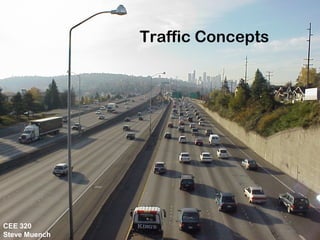
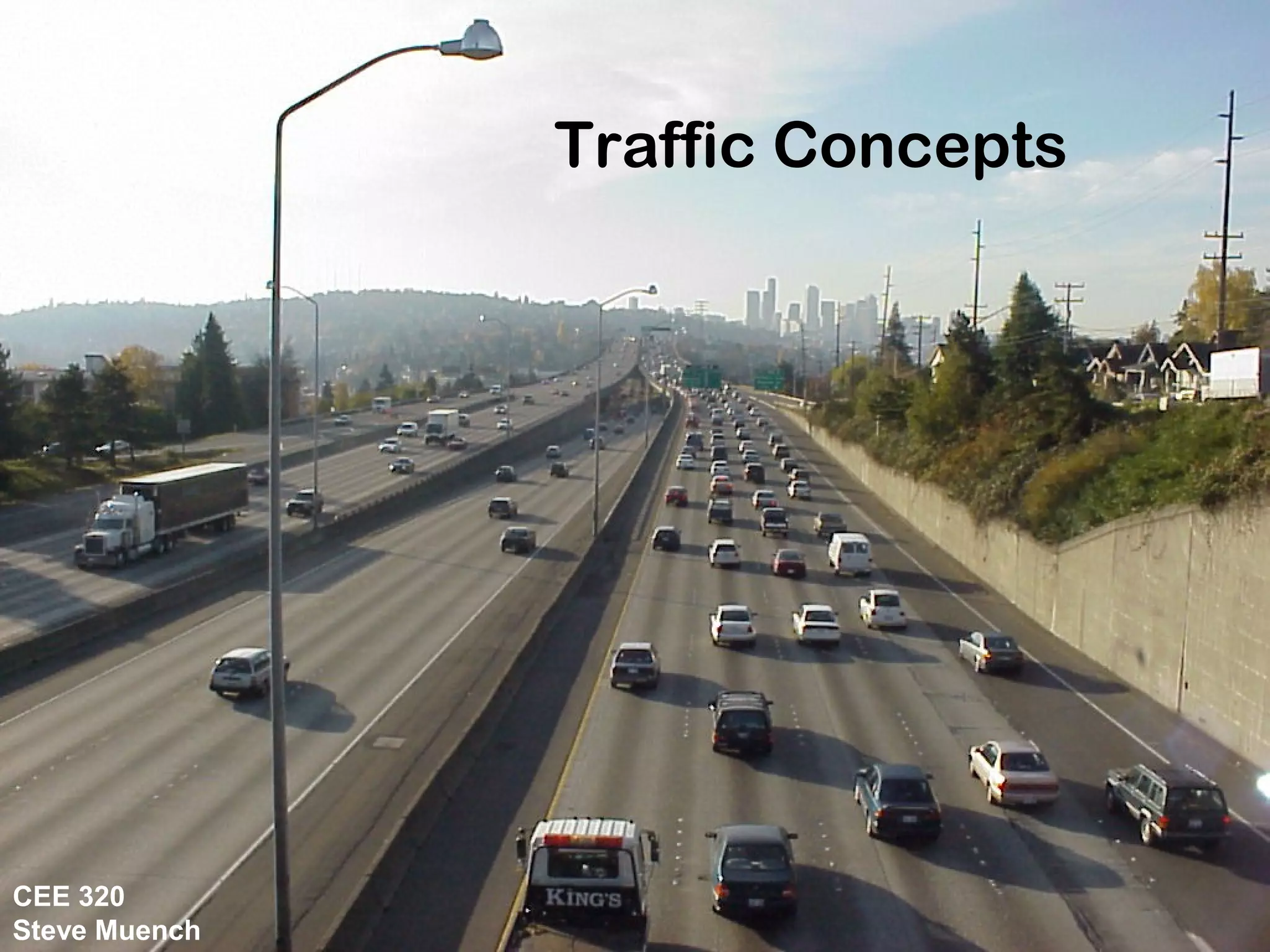
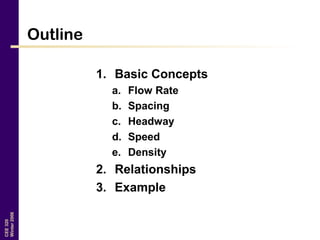
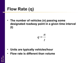
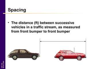
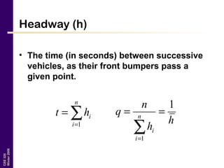
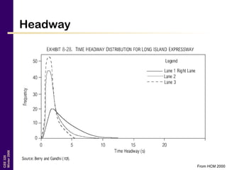
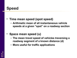
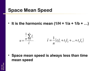
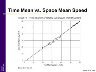
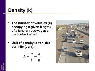
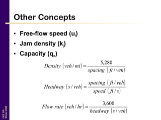
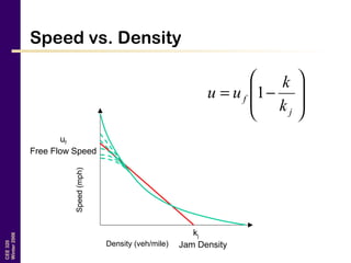
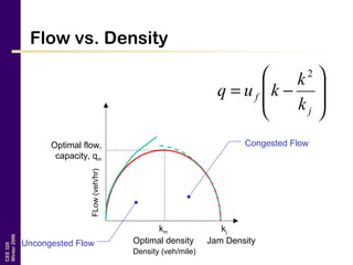
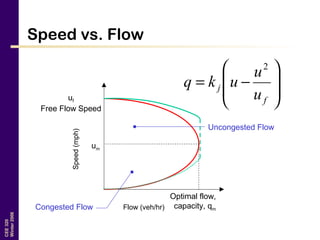
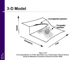
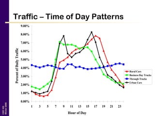
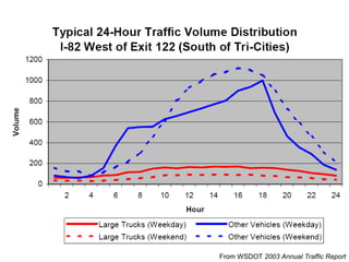
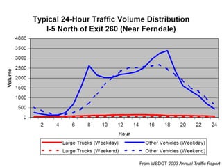
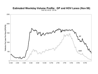
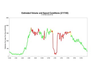
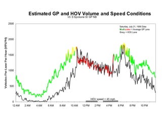
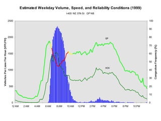
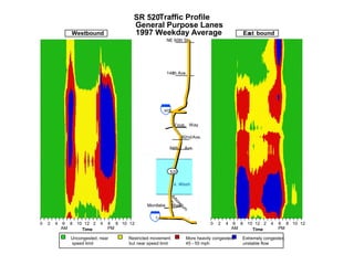

This document discusses key traffic concepts such as flow rate, spacing, headway, speed, and density. It defines these terms and explores the relationships between volume, speed, and density. Flow rate, spacing, headway, time mean speed and space mean speed are defined. Speed-density and flow-density relationships are presented, showing how traffic flow transitions from uncongested to congested states. Examples of traffic patterns by time of day and location are shown.


![11 Geometric Design of Railway Track [Vertical Alignment] (Railway Engineerin...](https://cdn.slidesharecdn.com/ss_thumbnails/geometricdesignofrailwaytrack-ii-200415172410-thumbnail.jpg?width=640&height=640&fit=bounds)
![10 Geometric Design of Railway Track [Horizontal Alignment] (Railway Engineer...](https://cdn.slidesharecdn.com/ss_thumbnails/geometricdesignofrailwaytrack-i-200415171932-thumbnail.jpg?width=640&height=640&fit=bounds)


![[Deck] What's New in Spark-Iceberg Integration via DSV2.pptx](https://cdn.slidesharecdn.com/ss_thumbnails/deckwhatsnewinspark-icebergintegrationviadsv2-260210005337-25955b12-thumbnail.jpg?width=640&height=640&fit=bounds)


