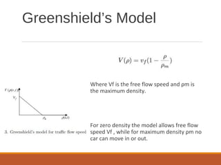
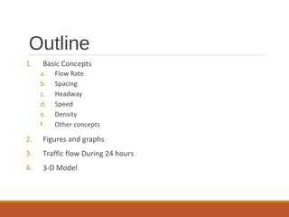
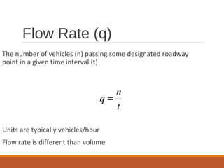
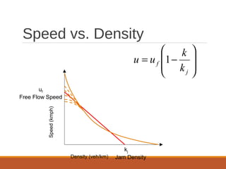
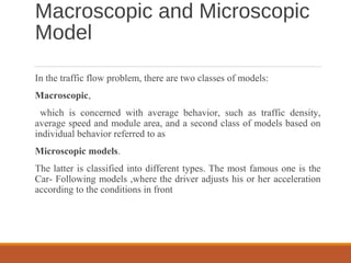
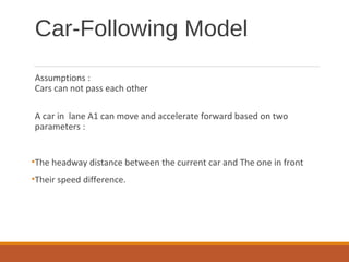
The document discusses traffic stream models. It describes two classes of traffic models: macroscopic models that examine average behaviors like density and speed, and microscopic models that examine individual behaviors like car-following models. The car-following model assumes cars cannot pass and a car's acceleration depends on the headway distance and speed difference of the car in front. Conservation laws state that the number of cars in a highway segment remains constant over time. Greenshield's model relates traffic speed to density, with free flow at low density and zero speed at maximum density. The document outlines concepts like flow rate, spacing, headway, density and speed-flow-density relationships.

1. Traffic stream models
Faris Jihad thyab
KKKA6783
Dr.Nur Izzi bin MD Yusoff

2. Introduction
Traffic flow is the study of interactions between vehicles, drivers and
infrastructure (including highways, signage and traffic control devices)
Interest in modeling traffic flow has been around since the appearance of
traffic jams. Ideally, if we can correctly predict the behavior of vehicle
flow given an initial set of data, then, in theory, adjusting the flow in
crucial areas can maximize the overall throughput of traffic along a
stretch of road. This is of particular interest in regions of high traffic
density, which may be caused by high volume peak time traffic,
accidents or closure of one or more lanes of the road

3. Macroscopic and Microscopic
Model
In the traffic flow problem, there are two classes of models:
Macroscopic,
which is concerned with average behavior, such as traffic density,
average speed and module area, and a second class of models based on
individual behavior referred to as
Microscopic models.
The latter is classified into different types. The most famous one is the
Car- Following models ,where the driver adjusts his or her acceleration
according to the conditions in front

4. Car-Following Model
Assumptions :
Cars can not pass each other
A car in lane A1 can move and accelerate forward based on two
parameters :
•The headway distance between the current car and The one in front
•Their speed difference.

5. Conservation Law
When physical quantities remain the same during some process, these
quantities are said to be conserved. Putting this principle into a
mathematical representation will make it possible to predict the densities
and velocities patterns at future time.
The number of cars in a segment of a highway [ x1,x2] are our physical
quantities, and the process is to keep them fixed (i.e., the number of cars
coming in equals the number of cars going out of the segment)

6. Greenshield’s Model
Where Vf is the free flow speed and ρm is
the maximum density.
For zero density the model allows free flow
speed Vf , while for maximum density ρm no
car can move in or out.

7. Outline
1. Basic Concepts
a. Flow Rate
b. Spacing
c. Headway
d. Speed
e. Density
f. Other concepts
2. Figures and graphs
3. Traffic flow During 24 hours
4. 3-D Model

8. Flow Rate (q)
t
n
q =
The number of vehicles (n) passing some designated roadway
point in a given time interval (t)
Units are typically vehicles/hour
Flow rate is different than volume

9. Spacing
The distance (ft) between successive vehicles in a traffic stream, as
measured from front bumper to front bumper

10. Headway (h)
∑=
=
n
i
iht
1
The time (in seconds) between successive vehicles, as their front bumpers
pass a given point.
h
h
n
q n
i
i
1
1
==
∑=

11. Speed
Time mean speed (spot speed)
◦ Arithmetic mean of all instantaneous vehicle speeds at a given “spot” on a
roadway section
Space mean speed (u)
◦ The mean travel speed of vehicles traversing a roadway segment of a known
distance (d)
◦ More useful for traffic applications

12. Density (k)
u
q
l
n
k ==
The number of vehicles
(n) occupying a given
length (l) of a lane or
roadway at a particular
instant
Unit of density is
vehicles per kilometer
(VpK).

13. Other Concepts
Free-flow speed (uf)
Jam density (kj)
Capacity (qm)
( )
( )vehftspacing
mivehDensity
/
280,5
/ =
( )
( )
( )sftspeed
vehftspacing
vehsHeadway
/
/
/ =
( )
( )vehsheadway
hrvehrateFlow
/
600,3
/ =

14. Speed vs. Density








−=
j
f
k
k
uu 1
Density (veh/km)
Speed(kmph)
kj
Jam Density
uf
Free Flow Speed

15. Flow vs. Density








−=
j
f
k
k
kuq
2
Density (veh/km)
FLow(veh/hr)
kj
Jam Density
Optimal flow,
capacity, qm
km
Optimal densityUncongested Flow
Congested Flow

16. Speed vs. Flow








−=
f
j
u
u
ukq
2
Flow (veh/hr)
Speed(kmph)
uf
Free Flow Speed
Optimal flow,
capacity, qm
Uncongested Flow
Congested Flow
um

17. Traffic – Time of Day
Patterns
0.00%
1.00%
2.00%
3.00%
4.00%
5.00%
6.00%
7.00%
8.00%
9.00%
1 3 5 7 9 11 13 15 17 19 21 23
Hour of Day
PercentofDailyTraffic
Rural Cars
Business Day Trucks
Through Trucks
Urban Cars

18. 3-D Model

19. Issues with Traffic Flow
Stop signs in wrong places
No signs available
One-way traffic
No pedestrian walkways
Weather

20. What helps?
Stops lights
Roundabouts
Pedestrian walkways
Bridges
Fast lanes
Bike lanes

21. Basic concept of ideal
model

22. Primary References
Mannering, F.L.; Kilareski, W.P. and Washburn, S.S. (2005). Principles of
Highway Engineering and Traffic Analysis, Third Edition. Chapter 5
Transportation Research Board. (2000). Highway Capacity Manual 2000.
National Research Council, Washington, D.C.