Department of CivilEngineering, NIT Srinagar
A presentation on
Presented By:
Dr. Abdullah Ahmad
Assistant Professor
1
2.
❖ Traffic Volume(q)
o It is the number of vehicles that pass a given point during
specified unit of time.
o It is measured in vehicle per hour.
o It is represented by ‘q’
o q= (N *3600)/t
2
3.
❖ Traffic Density(k)
o It is the number of vehicle occupying a unit length of lane of
roadway at a given instant of time.
o It is measured in vehicle per kilometre.
o It is represented by ‘K’
o K= N/L
o Where,
o N=No. of vehicles over a stretch of roadway (L) i.e. vehicles
per kilometer
3
4.
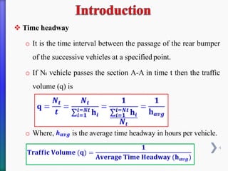
❖ Time headway
oIt is the time interval between the passage of the rear bumper
of the successive vehicles at a specified point.
o If Nt vehicle passes the section A-A in time t then the traffic
volume (q) is
o Where, is the average time headway in hours per vehicle.
4
5.
❖ Space headway
oThe distance between the rear bumper of the successive
vehicles is called as space headway.
o If Nx number of vehicle occupying a length x of a lane of
roadway then traffic density is.
o Where, is the average space headway in km per vehicle.
5
6.
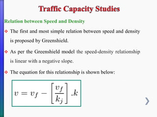
Relation between Speedand Density
❖ The first and most simple relation between speed and density
is proposed by Greenshield.
❖ As per the Greenshield model the speed-density relationship
is linear with a negative slope.
❖ The equation for this relationship is shown below:
7.
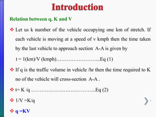
Relation between q,K and V
❖ Let us k number of the vehicle occupying one km of stretch. If
each vehicle is moving at a speed of v kmph then the time taken
by the last vehicle to approach section A-A is given by
t = 1(km)/V (kmph)……………………..Eq (1)
❖ If q is the traffic volume in vehicle /hr then the time required to K
no of the vehicle will cross-section A-A .
❖ t= K /q ………………………………..Eq (2)
❖ 1/V =K/q
❖ q =KV
7
8.
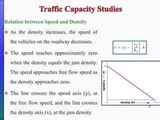
Relation between Speedand Density
❖ As the density increases, the speed of
the vehicles on the roadway decreases.
❖ The speed reaches approximately zero
when the density equals the jam density.
The speed approaches free flow speed as
the density approaches zero.
❖ The line crosses the speed axis (y), at
the free flow speed, and the line crosses
the density axis (x), at the jam density.
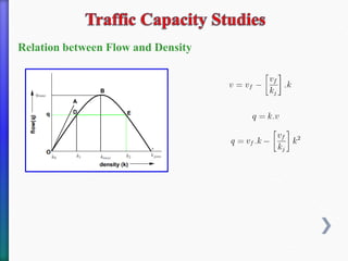
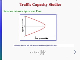
Relation between Speedand Flow
Similarly we can find the relation between speed and flow.
11.
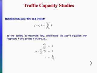
To find densityat maximum flow, differentiate the above equation with
respect to k and equate it to zero. ie.,
Relation between Flow and Density
12.
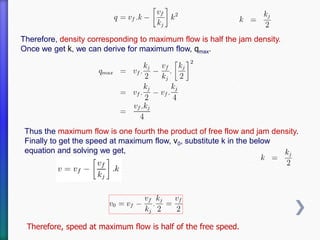
Therefore, density correspondingto maximum flow is half the jam density.
Once we get k, we can derive for maximum flow, qmax.
Thus the maximum flow is one fourth the product of free flow and jam density.
Finally to get the speed at maximum flow, v0, substitute k in the below
equation and solving we get,
Therefore, speed at maximum flow is half of the free speed.
13.
Traffic Capacity:
❖ Theability of a roadway to accommodate traffic volume.
❖ It is expressed as the maximum number of vehicles in a lane or a
road that can pass a given point in unit time, usually an hour.
❖ It is expressed as vehicle per hour per lane.
14.
Traffic Capacity:
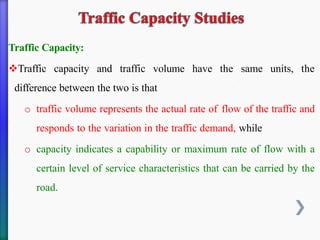
❖Traffic capacityand traffic volume have the same units, the
difference between the two is that
o traffic volume represents the actual rate of flow of the traffic and
responds to the variation in the traffic demand, while
o capacity indicates a capability or maximum rate of flow with a
certain level of service characteristics that can be carried by the
road.
15.
Traffic Capacity:
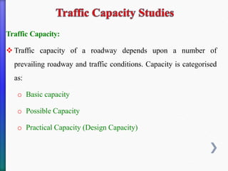
❖ Trafficcapacity of a roadway depends upon a number of
prevailing roadway and traffic conditions. Capacity is categorised
as:
o Basic capacity
o Possible Capacity
o Practical Capacity (Design Capacity)
16.
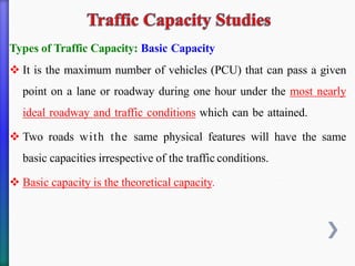
Types of TrafficCapacity: Basic Capacity
❖ It is the maximum number of vehicles (PCU) that can pass a given
point on a lane or roadway during one hour under the most nearly
ideal roadway and traffic conditions which can be attained.
❖ Two roads with the same physical features will have the same
basic capacities irrespective of the traffic conditions.
❖ Basic capacity is the theoretical capacity.
17.
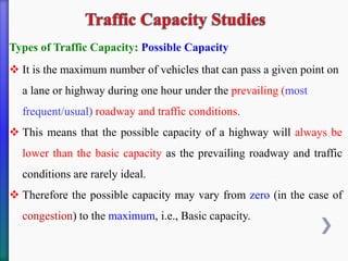
Types of TrafficCapacity: Possible Capacity
❖ It is the maximum number of vehicles that can pass a given point on
a lane or highway during one hour under the prevailing (most
frequent/usual) roadway and traffic conditions.
❖ This means that the possible capacity of a highway will always be
lower than the basic capacity as the prevailing roadway and traffic
conditions are rarely ideal.
❖ Therefore the possible capacity may vary from zero (in the case of
congestion) to the maximum, i.e., Basic capacity.
18.
Types of TrafficCapacity: Practical Capacity:
❖ For design purpose we neither use basic capacity or possible
capacity as they represents the two extreme cases of roadway and
traffic condition. Hence we have use another types of capacity called
practical capacity.
❖ It is the maximum number of vehicles that can pass a given point on
a lane or roadway during one hour without traffic density being so
great as to cause unreasonable delay, hazard, or restriction to the
driver's freedom to manoeuvre under the prevailing roadway and
traffic conditions.
19.
Types of TrafficCapacity: Practical Capacity
❖ It is the capacity which is of primary interest to the designers who
strive to provide adequate highway facilities hence this is also called
the design capacity.
❖ It is the practical capacity or a smaller value determined for use in
designing the highway to accommodate the design hourly volume
(D.H.V).
❖ It is a term, normally, applied to existing highways.
20.
Calculation of MaxTheoretical Capacity from Space Headway (S):
❖ The theoretical capacity is the maximum number of vehicles passing
any point in one hour per lane.
❖ It depends upon the average length of the vehicle and the average
spacing of the moving vehicles. Mathematically, theoretical capacity
of a single lane,
V = Design Speed of the vehicle in kmph
S = Centre to center spacing of moving vehicle
21.
Calculation of MaxTheoretical Capacity from Space Headway (S):
❖ Thus the theoretical capacity depends upon Speed and Spacing.
❖ Spacing is governed by the safe stopping distance required to be the
rear vehicle in case the vehicle ahead stops suddenly.
❖ Numerically spacing is given by,
❖ S = Sg + L
❖ Where,
o Sg =the space gap (Head to rear) between the vehicles
o L = the average length of the vehicle, both combined make the
center to center spacing of the vehicles.
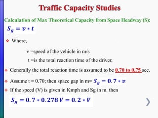
22.
Calculation of MaxTheoretical Capacity from Space Headway (S):
❖ Where,
v =speed of the vehicle in m/s
t =is the total reaction time of the driver,
❖ Generally the total reaction time is assumed to be 0.70 to 0.75 sec.
❖ Assume t = 0.70; then space gap in m=
❖ If the speed (V) is given in Kmph and Sg in m. then
23.
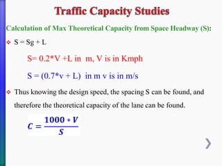
Calculation of MaxTheoretical Capacity from Space Headway (S):
❖ S = Sg + L
S= 0.2*V +L in m, V is in Kmph
S = (0.7*v + L) in m v is in m/s
❖ Thus knowing the design speed, the spacing S can be found, and
therefore the theoretical capacity of the lane can be found.
24.
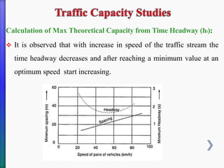
Calculation of MaxTheoretical Capacity from Time Headway (ht):
❖ It is observed that with increase in speed of the traffic stream the
time headway decreases and after reaching a minimum value at an
optimum speed start increasing.
25.
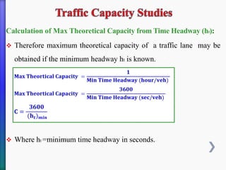
Calculation of MaxTheoretical Capacity from Time Headway (ht):
❖ Therefore maximum theoretical capacity of a traffic lane may be
obtained if the minimum headway ht is known.
❖ Where ht =minimum time headway in seconds.
26.
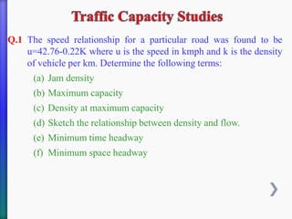
Q.1 The speedrelationship for a particular road was found to be
u=42.76-0.22K where u is the speed in kmph and k is the density
of vehicle per km. Determine the following terms:
(a) Jam density
(b) Maximum capacity
(c) Density at maximum capacity
(d) Sketch the relationship between density and flow.
(e) Minimum time headway
(f) Minimum space headway
27.
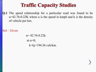
Q.1 The speedrelationship for a particular road was found to be
u=42.76-0.22K where u is the speed in kmph and k is the density
of vehicle per km.
Sol : Given
u= 42.76-0.22k
at u=0;
k=kj=194.36 veh/km.
28.
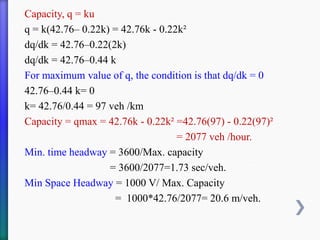
Capacity, q =ku
q = k(42.76– 0.22k) = 42.76k - 0.22k²
dq/dk = 42.76–0.22(2k)
dq/dk = 42.76–0.44 k
For maximum value of q, the condition is that dq/dk = 0
42.76–0.44 k= 0
k= 42.76/0.44 = 97 veh /km
Capacity = qmax = 42.76k - 0.22k² =42.76(97) - 0.22(97)²
= 2077 veh /hour.
Min. time headway = 3600/Max. capacity
= 3600/2077=1.73 sec/veh.
Min Space Headway = 1000 V/ Max. Capacity
= 1000*42.76/2077= 20.6 m/veh.
29.
Q.2 The freemean speed on a roadway is found to be
80 kmph. Under stopped conditions, the average
spacing is 6.9 m. Determine the jam density and
maximum flow.
30.
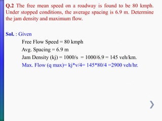
Q.2 The freemean speed on a roadway is found to be 80 kmph.
Under stopped conditions, the average spacing is 6.9 m. Determine
the jam density and maximum flow.
Sol. : Given
Free Flow Speed = 80 kmph
Avg. Spacing = 6.9 m
Jam Density (kj) = 1000/s = 1000/6.9 = 145 veh/km.
Max. Flow (q max)= kj*v/4= 145*80/4 =2900 veh/hr.
31.
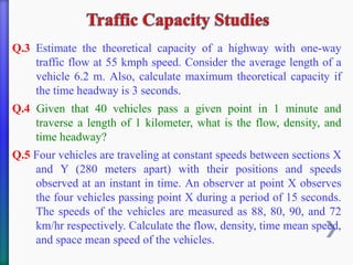
Q.3 Estimate thetheoretical capacity of a highway with one-way
traffic flow at 55 kmph speed. Consider the average length of a
vehicle 6.2 m. Also, calculate maximum theoretical capacity if
the time headway is 3 seconds.
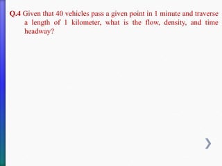
Q.4 Given that 40 vehicles pass a given point in 1 minute and
traverse a length of 1 kilometer, what is the flow, density, and
time headway?
Q.5 Four vehicles are traveling at constant speeds between sections X
and Y (280 meters apart) with their positions and speeds
observed at an instant in time. An observer at point X observes
the four vehicles passing point X during a period of 15 seconds.
The speeds of the vehicles are measured as 88, 80, 90, and 72
km/hr respectively. Calculate the flow, density, time mean speed,
and space mean speed of the vehicles.
32.
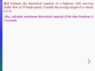
Q.3 Estimate thetheoretical capacity of a highway with one-way
traffic flow at 55 kmph speed. Consider the average length of a vehicle
6.2 m.
Also, calculate maximum theoretical capacity if the time headway is
3 seconds.
33.
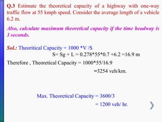
Q.3 Estimate thetheoretical capacity of a highway with one-way
traffic flow at 55 kmph speed. Consider the average length of a vehicle
6.2 m.
Also, calculate maximum theoretical capacity if the time headway is
3 seconds.
Sol.: Theoritical Capacity = 1000 *V /S
S= Sg + L = 0.278*55*0.7 +6.2 =16.9 m
Therefore , Theoretical Capacity = 1000*55/16.9
=3254 veh/km.
Max. Theoretical Capacity = 3600/3
= 1200 veh/ hr.
34.
Q.4 Given that40 vehicles pass a given point in 1 minute and traverse
a length of 1 kilometer, what is the flow, density, and time
headway?
35.
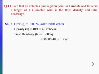
Q.4 Given that40 vehicles pass a given point in 1 minute and traverse
a length of 1 kilometer, what is the flow, density, and time
headway?
Sol. : Flow (q) = 3600*40/60 = 2400 Veh/hr.
Density (k) = 40/1 = 40 veh/km.
Time Headway (ht) = 3600/q
= 3600/2400= 1.5 sec.
36.
36
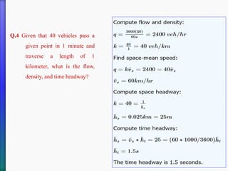
Q.4 Given that40 vehicles pass a
given point in 1 minute and
traverse a length of 1
kilometer, what is the flow,
density, and time headway?
37.
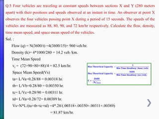
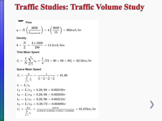
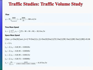
Q.5 Four vehiclesare traveling at constant speeds between sections X and Y (280 meters
apart) with their positions and speeds observed at an instant in time. An observer at point X
observes the four vehicles passing point X during a period of 15 seconds. The speeds of the
vehicles are measured as 88, 80, 90, and 72 km/hr respectively. Calculate the flow, density,
time mean speed, and space mean speed of the vehicles.
Sol. :
Flow (q) = N(3600/t) =4(3600/15)= 960 veh/hr.
Density (k)= 4*1000/280 = 14.2 veh /km.
Time Mean Speed
vt = (72+90+80+88)/4 = 82.5 km/hr.
Space Mean Speed(Vs)
ta= L/Va=0.28/88 = 0.00318 hr.
tb= L/Vb=0.28/80 = 0.00350 hr.
tc= L/Vc=0.28/90 = 0.00311 hr.
td= L/Va=0.28/72= 0.00389 hr.
Vs=N*L/(ta+tb+tc+td) =4*.28/(.00318+.00350+.00311+.00389)
= 81.87 km/hr.
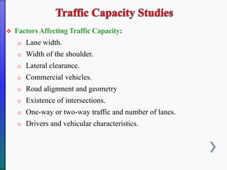
❖ Factors AffectingTraffic Capacity:
o Lane width.
o Width of the shoulder.
o Lateral clearance.
o Commercial vehicles.
o Road alignment and geometry
o Existence of intersections.
o One-way or two-way traffic and number of lanes.
o Drivers and vehicular characteristics.
41.
❖ Factors AffectingTraffic Capacity:
o Lane width.
o Width of the shoulder.
o Lateral clearance.
o Commercial vehicles.
o Road alignment and geometry
o Existence of intersections.
o One-way or two-way traffic and number of lanes.
o Drivers and vehicular characteristics.
42.
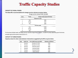
CAPACITY OF RURALROADS:
The latest IRC recommendations for design service volumes are given below:
For four-lane divided roads, the design service volumes range from 47,000 to 1, 05,000 PCU/day depending upon the terrain,
shoulder-type and the level of service (B or C).
CAPACITY OF URBAN ROADS :
Capacity values for urban roads (between intersections suggested by the IRC are given below:
43.
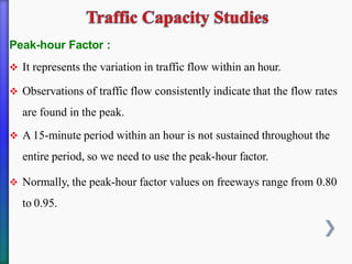
Peak-hour Factor :
❖It represents the variation in traffic flow within an hour.
❖ Observations of traffic flow consistently indicate that the flow rates
are found in the peak.
❖ A 15-minute period within an hour is not sustained throughout the
entire period, so we need to use the peak-hour factor.
❖ Normally, the peak-hour factor values on freeways range from 0.80
to 0.95.
44.
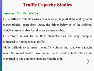
Passenger Car Unit(PCU) :
❖The different vehicle classes have a wide range of static and dynamic
characteristics; apart from these, the driver behavior of the different
vehicle classes is also found to vary considerably.
❖Therefore, mixed traffic flow characteristics are very complex
compared to homogeneous traffic.
❖It is difficult to estimate the traffic volume and roadway capacity
under the mixed traffic flow unless the different vehicle classes are
converted to one common standard vehicle unit.
45.
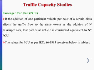
Passenger Car Unit(PCU) :
❖If the addition of one particular vehicle per hour of a certain class
affects the traffic flow to the same extent as the addition of N
passenger cars, that particular vehicle is considered equivalent to N*
PCU.
❖The values for PCU as per IRC: 86-1983 are given below in tables :
46.
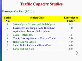
Passenger Car Unit(PCU) :
Serial
No.
Vehicle Class Equivalence
Factor
1 Motor Cycle, Scooter and Pedal Cycle 0.5
2 Passenger Car, Tempo, Auto Rickshaw,
Agricultural Tractor, Pick-Up Van
1.0
3 Cycle – Rickshaw 1.5
4 Truck, Bus, Agricultural Tractor- Trailer 3.0
5 Horse-Drawn Vehicle 4.0
6 Small Bullock-Cart and Hand-Cart 6.0
7 Large Bullock-Cart 8.0
47.
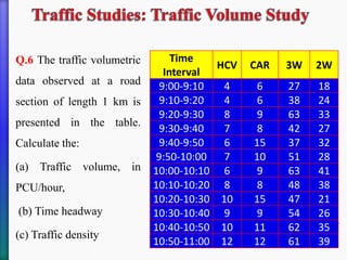
Q.6 The trafficvolumetric
data observed at a road
section of length 1 km is
presented in the table.
Calculate the:
(a) Traffic volume, in
PCU/hour,
(b) Time headway
(c) Traffic density
47
Time
Interval
HCV CAR 3W 2W
9:00-9:10 4 6 27 18
9:10-9:20 4 6 38 24
9:20-9:30 8 9 63 33
9:30-9:40 7 8 42 27
9:40-9:50 6 15 37 32
9:50-10:00 7 10 51 28
10:00-10:10 6 9 63 41
10:10-10:20 8 8 48 38
10:20-10:30 10 15 47 21
10:30-10:40 9 9 54 26
10:40-10:50 10 11 62 35
10:50-11:00 12 12 61 39
48.
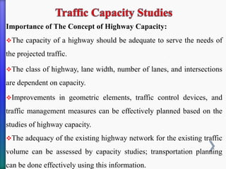
Importance of TheConcept of Highway Capacity:
❖The capacity of a highway should be adequate to serve the needs of
the projected traffic.
❖The class of highway, lane width, number of lanes, and intersections
are dependent on capacity.
❖Improvements in geometric elements, traffic control devices, and
traffic management measures can be effectively planned based on the
studies of highway capacity.
❖The adequacy of the existing highway network for the existing traffic
volume can be assessed by capacity studies; transportation planning
can be done effectively using this information.
49.
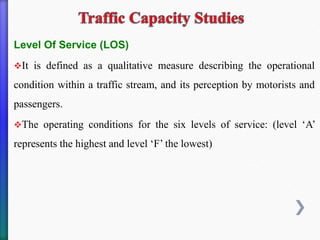
Level Of Service(LOS)
❖It is defined as a qualitative measure describing the operational
condition within a traffic stream, and its perception by motorists and
passengers.
❖The operating conditions for the six levels of service: (level ‘A’
represents the highest and level ‘F’ the lowest)
50.
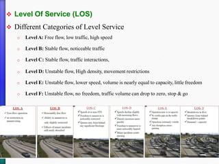
❖ Level OfService (LOS)
❖ Different Categories of Level Service
o LevelA: Free flow, low traffic, high speed
o Level B: Stable flow, noticeable traffic
o Level C: Stable flow, traffic interactions,
o Level D: Unstable flow, High density, movement restrictions
o Level E: Unstable flow, lower speed, volume is nearly equal to capacity, little freedom
o Level F: Unstable flow, no freedom, traffic volume can drop to zero, stop & go
51.
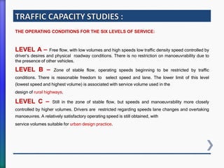
THE OPERATING CONDITIONSFOR THE SIX LEVELS OF SERVICE:
LEVEL A – Free flow, with low volumes and high speeds low traffic density speed controlled by
driver’s desires and physical roadway conditions. There is no restriction on manoeuvrability due to
the presence of other vehicles.
LEVEL B – Zone of stable flow, operating speeds beginning to be restricted by traffic
conditions. There is reasonable freedom to select speed and lane. The lower limit of this level
(lowest speed and highest volume) is associated with service volume used in the
design of rural highways.
LEVEL C – Still in the zone of stable flow, but speeds and manoeuvrability more closely
controlled by higher volumes. Drivers are restricted regarding speeds lane changes and overtaking
manoeuvres. A relatively satisfactory operating speed is still obtained, with
service volumes suitable for urban design practice.
52.
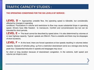
THE OPERATING CONDITIONSFOR THE SIX LEVELS OF SERVICE:
LEVEL D – Approaches unstable flow, the operating speed is tolerable, but considerably
affected by changes in operating
conditions. Fluctuations in volume and restrictions to flow may cause substantial drops in operating
speed. Drivers have little freedom to manoeuvre. Comfort and convenienceare low but can be
tolerated for short periods.
LEVEL E – This level cannot be described by speed alone. It is also determined by volumes at
or near highway capacity. Typical speeds are 50km/h. Flow is unstable and there may be stoppages
of short durations.
LEVEL F – At this level, there are forced operations at low speeds resulting in volumes below
capacity. Queues of vehicles piling up from a restriction downstream serve as a storage area during
peak hour. Substantial reduction in speeds and stoppages may occur
for short or long duration because of downstream congestion. In the extreme, both speed and
volume can drops to zero.
53.
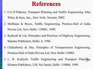
1. CA O’Flaherty,Transport Planning and Traffic Engineering, John
Wiley & Sons, Inc., New York; Toronto, 2002.
2. McShane & Roess, Traffic Engineering, Prentice‐Hall of India
Private Ltd, New Delhi‐ 110001, 1990.
3. Kadiyali & Lal, Principles and Practices of Highway Engineering,
Khanna Publishers, Delhi‐ 6, 1996.
4. Chakarborty & Das, Principles of Transportation Engineering,
Prentice‐Hall of India Private Ltd, New Delhi‐110001.
5. L. R. Kadiyali, Traffic Engineering and Transport Planning,
Khanna Publishers, 2‐B, Nai Sarak, Delhi‐ 110006, 1999.
53