traffic engg

1. Traffic Flow
Fundamental Parameters & Diagrams
Centre for Transportation Research (CTR)
Department of Civil Engineering
NATIONAL INSTITUTE OF TECHNOLOGY CALICUT
NITC P.O., CALICUT – 673601
M.V.L.R. Anjaneyulu
mvlr@nitc.ac.in

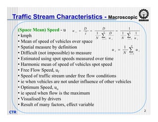
2. (Space Mean) Speed - u
• kmph
• Mean of speed of vehicles over space
• Spatial measure by definition
• Difficult (not impossible) to measure
• Estimated using spot speeds measured over time
Traffic Stream Characteristics - Macroscopic



N
i
i
t u
N
u
1
1

 



 N
i i
N
i i
s
u
N
u
D
N
D
t
D
u
1
1
1
1
1
1
CTR 2
• Estimated using spot speeds measured over time
• Harmonic mean of speed of vehicles spot speed
• Free Flow Speed, uf
• Speed of traffic stream under free flow conditions
• ie when vehicles are not under influence of other vehicles
• Optimum Speed, uo
• ie speed when flow is the maximum
• Visualised by drivers
• Result of many factors, effect variable

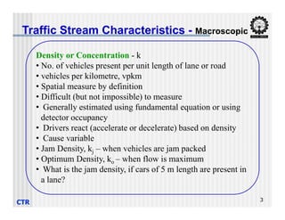
3. Density or Concentration - k
• No. of vehicles present per unit length of lane or road
• vehicles per kilometre, vpkm
• Spatial measure by definition
• Difficult (but not impossible) to measure
• Generally estimated using fundamental equation or using
Traffic Stream Characteristics - Macroscopic
CTR 3
• Generally estimated using fundamental equation or using
detector occupancy
• Drivers react (accelerate or decelerate) based on density
• Cause variable
• Jam Density, kj – when vehicles are jam packed
• Optimum Density, ko – when flow is maximum
• What is the jam density, if cars of 5 m length are present in
a lane?

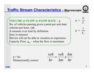
4. VOLUME or FLOW or FLOW RATE – q
No. of vehicles passing given a point per unit time
vehicles per hour, vph
A measure over time by definition
Easy to measure
Drivers will not be able to visualise or experience
Traffic Stream Characteristics - Macroscopic
T
N
q 
t
h
q
1

CTR 4
Drivers will not be able to visualise or experience
Capacity Flow, qm – when the flow is maximum
hr
km
x
km
veh
hr
veh

q = ku
Dimensionally correct

5. Traffic Stream Characteristics - Microscopic
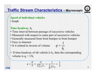
Speed of individual vehicles
• kmph
Time headway, ht
• Time interval between passage of successive vehicles
• Measured with respect to same part of successive vehicles
• Generally measured from front bumper to front bumper
CTR 5
• Generally measured from front bumper to front bumper
• Easy to measure
• It is related to inverse of volume
• If time headway of ith vehicle is hi, then the corresponding
volume is qi = 1/hi
t
h
q
1


6. Traffic Stream Characteristics - Microscopic
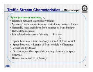
Space (distance) headway, hs
• Distance between successive vehicles
• Measured with respect to same part of successive vehicles
• Generally measured from front bumper to front bumper
• Difficult to measure
• It is related to inverse of density
h
k
1

CTR 6
• Space headway = time headway x speed of front vehicle
• Space headway = Length of front vehicle + Clearance
• Visualised by drivers
• Drivers adjust their speed depending clearance or space
headway
• Drivers are sensitive to density
s
h
k 

7. Time space diagram
CTR 7

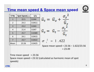
8. V No Spot Speed, u 1/u
1 22.5 0.044
2 24.3 0.0411
3 23.2 0.043
4 21.4 0.047
5 25.7 0.0389
6 24.1 0.0415
Time mean speed & Space mean speed
CTR 8
6 24.1 0.0415
7 23.7 0.0422
Mean 23.56 0.0425
Time mean speed = 23.56
Space mean speed = 23.52 (calculated as harmonic mean of spot
speeds)
622
.
1
2

t

Space mean speed = 23.56 – 1.622/23.56
= 23.49

9. A
C
D
60 m
11 m/sec
P
0 m
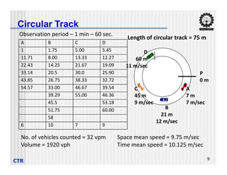
Length of circular track = 75 m
Observation period – 1 min – 60 sec.
A B C D
1 1.75 5.00 5.45
11.71 8.00 13.33 12.27
22.43 14.25 21.67 19.09
33.14 20.5 30.0 25.90
43.85 26.75 38.33 32.72
54.57 33.00 46.67 39.54
Circular Track
CTR 9
A
7 m
7 m/sec
B
21 m
12 m/sec
C
45 m
9 m/sec
54.57 33.00 46.67 39.54
39.29 55.00 46.36
45.5 53.18
51.75 60.00
58
6 10 7 9
No. of vehicles counted = 32 vpm
Volume = 1920 vph
Space mean speed = 9.75 m/sec
Time mean speed = 10.125 m/sec

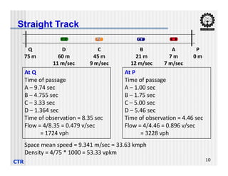
10. A
7 m
7 m/sec
B
21 m
12 m/sec
C
45 m
9 m/sec
D
60 m
11 m/sec
P
0 m
Q
75 m
At P
Time of passage
A – 1.00 sec
At Q
Time of passage
A – 9.74 sec
Straight Track
CTR 10
A – 1.00 sec
B – 1.75 sec
C – 5.00 sec
D – 5.46 sec
Time of observation = 4.46 sec
Flow = 4/4.46 = 0.896 v/sec
= 3228 vph
A – 9.74 sec
B – 4.755 sec
C – 3.33 sec
D – 1.364 sec
Time of observation = 8.35 sec
Flow = 4/8.35 = 0.479 v/sec
= 1724 vph
Space mean speed = 9.341 m/sec = 33.63 kmph
Density = 4/75 * 1000 = 53.33 vpkm

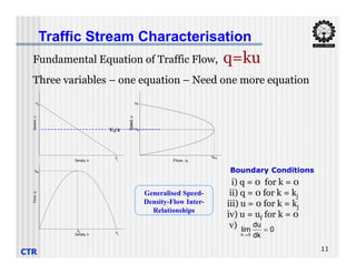
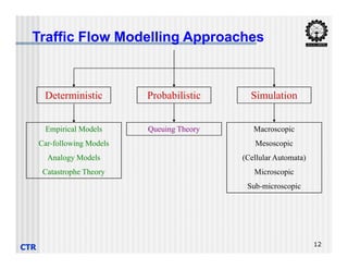
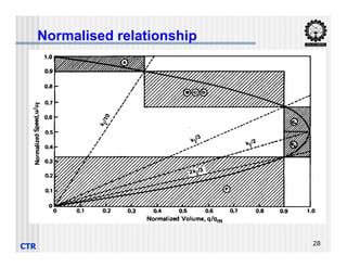
11. Traffic Stream Characterisation
Fundamental Equation of Traffic Flow, q=ku
Three variables – one equation – Need one more equation
Speed,
u
u
f
Speed,
u
uf
uo
Uf/2
CTR 11
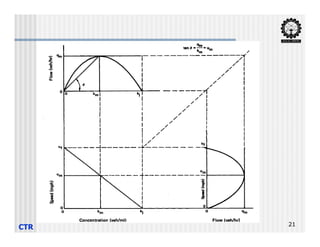
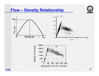
Generalised Speed-
Density-Flow Inter-
Relationships
Density, k
k
j Flow, q
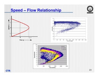
qm
Density, k
Flow,
q
kj
qm
ko
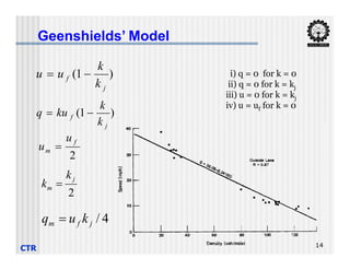
i) q = 0 for k = 0
ii) q = 0 for k = kj
iii) u = 0 for k = kj
iv) u = uf for k = 0
v) lim
k
du
dk


0
0
Boundary Conditions

12. Deterministic Probabilistic Simulation
Empirical Models Queuing Theory Macroscopic
Traffic Flow Modelling Approaches
CTR 12
Car-following Models
Analogy Models
Catastrophe Theory
Mesoscopic
(Cellular Automata)
Microscopic
Sub-microscopic

13. Traffic Stream Charcterisation
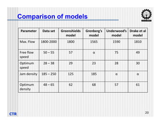
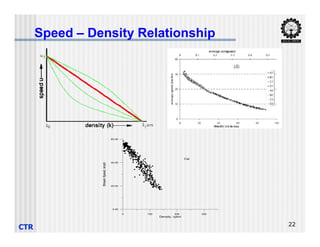
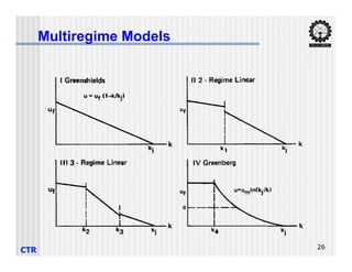
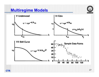
Speed – Density relationship is preferred
• Greenshields model
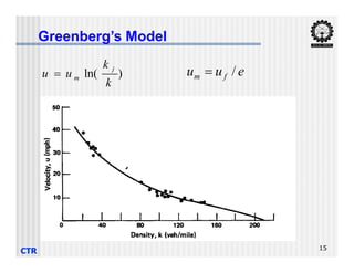
• Greenberg’s model
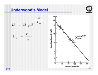
• Underwood’s model
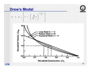
• Drew’s model
CTR 13
• Drew’s model
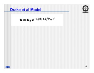
• Drake et al model

14. Geenshields’ Model
u
)
1
(
j
f
k
k
ku
q 

)
1
(
j
f
k
k
u
u 
 i) q = 0 for k = 0
ii) q = 0 for k = kj
iii) u = 0 for k = kj
iv) u = uf for k = 0
CTR 14
2
f
m
u
u 
2
j
m
k
k 
4
/
j
f
m k
u
q 

15. Greenberg’s Model
)
ln(
k
k
u
u
j
m
 e
u
u f
m /

CTR 15

16. Underwood’s Model
m
k
k
f e
u
u


e
k
k
j
m 
CTR 16
e
k m 

17. Pipes-Munjal Model
CTR 17

18. Drake et al Model
CTR 18

19. Drew’s Model





















2
1
1
n
j
f
k
k
u
u
CTR 19

20. Parameter Data set Greenshields
model
Grenberg’s
model
Underwood’s
model
Drake et al
model
Max. Flow 1800-2000 1800 1565 1590 1810
Free flow
speed
50 – 55 57 α 75 49
Optimum 28 – 38 29 23 28 30
Comparison of models
CTR 20
Optimum
speed
28 – 38 29 23 28 30
Jam density 185 – 250 125 185 α α
Optimum
density
48 – 65 62 68 57 61

21. CTR 21

22. Speed – Density Relationship
CTR 22
0 100 200 300
Density, vpkm
0.00
20.00
40.00
60.00
Stream
Speed,
kmph
Car

23. Speed – Flow Relationship
CTR 23

24. Flow – Density Relationship
CTR 24

25. Multiregime Models
CTR 25

26. Multiregime Models
CTR 26

27. Multiregime Models
CTR 27

28. Normalised relationship
CTR 28

29. Effect of interval size
CTR 29

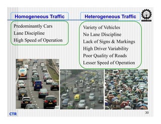
30. Predominantly Cars
Lane Discipline
High Speed of Operation
Variety of Vehicles
No Lane Discipline
Lack of Signs & Markings
High Driver Variability
Poor Quality of Roads
Lesser Speed of Operation
Homogeneous Traffic Heterogeneous Traffic
CTR 30
Lesser Speed of Operation

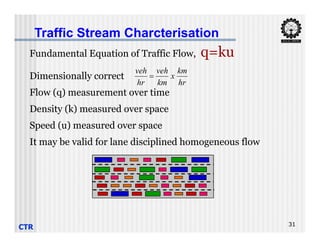
31. Traffic Stream Charcterisation
Fundamental Equation of Traffic Flow, q=ku
Dimensionally correct
Flow (q) measurement over time
Density (k) measured over space
Speed (u) measured over space
hr
km
x
km
veh
hr
veh

CTR 31
Speed (u) measured over space
It may be valid for lane disciplined homogeneous flow

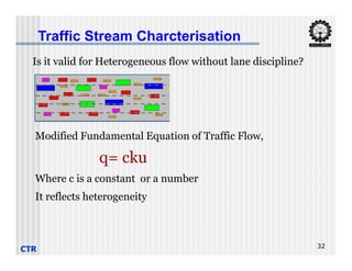
32. Is it valid for Heterogeneous flow without lane discipline?
Modified Fundamental Equation of Traffic Flow,
Traffic Stream Charcterisation
CTR 32
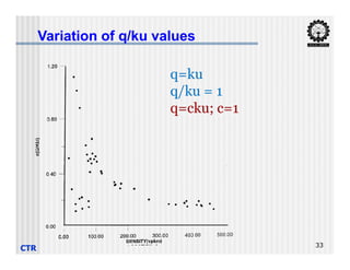
Modified Fundamental Equation of Traffic Flow,
q= cku
Where c is a constant or a number
It reflects heterogeneity

33. q=ku
q/ku = 1
q=cku; c=1
Variation of q/ku values
CTR 33

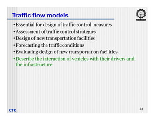
34. • Essential for design of traffic control measures
• Assessment of traffic control strategies
• Design of new transportation facilities
• Forecasting the traffic conditions
• Evaluating design of new transportation facilities
• Describe the interaction of vehicles with their drivers and
Traffic flow models
CTR 34
• Describe the interaction of vehicles with their drivers and
the infrastructure

35. Thank You