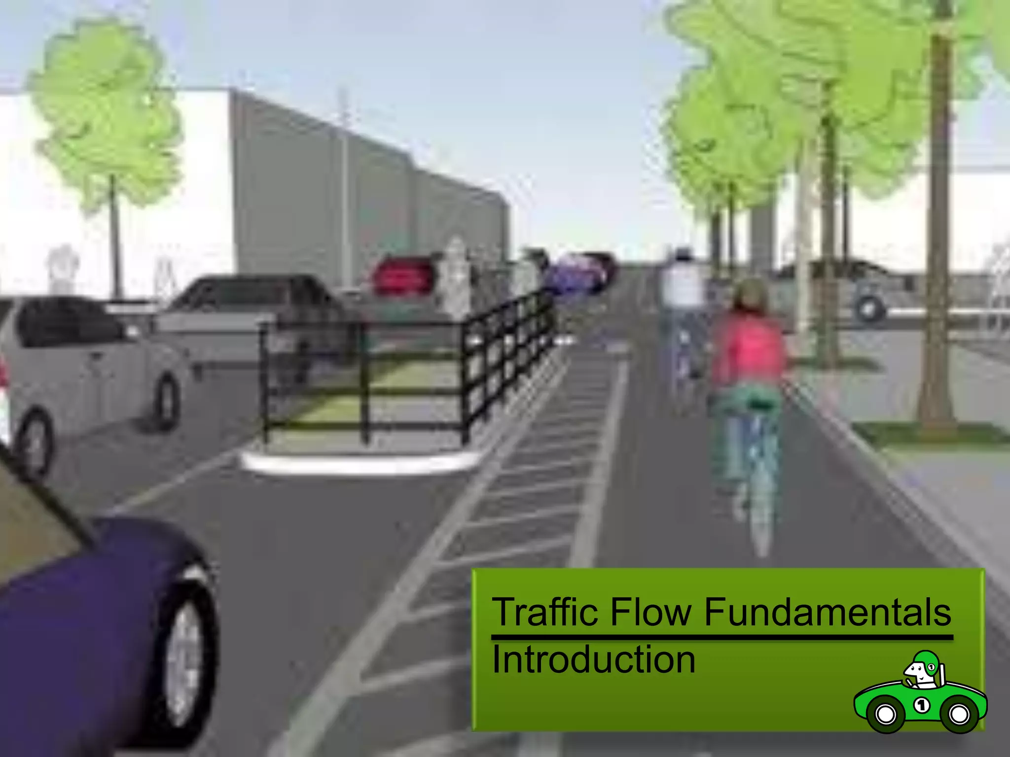
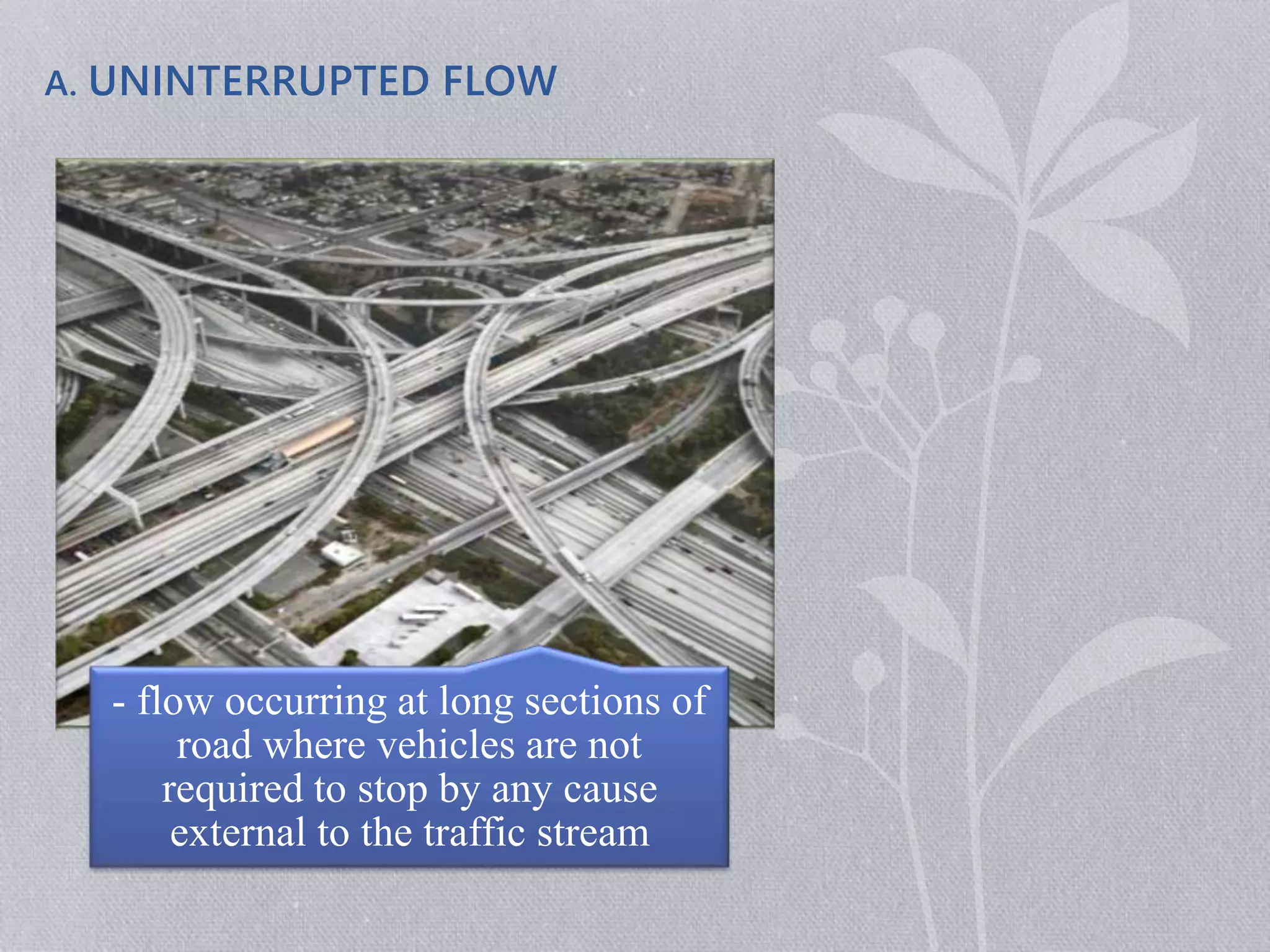
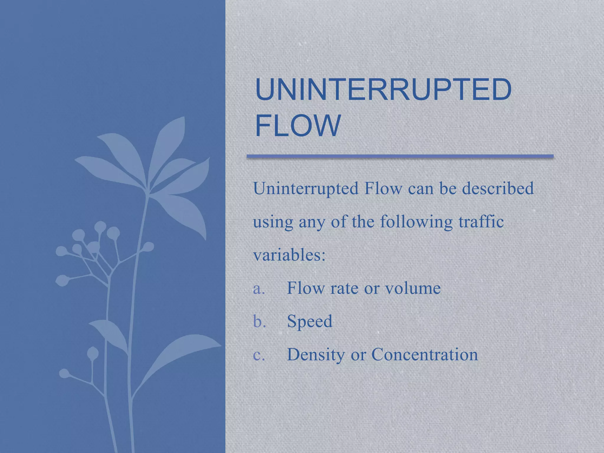
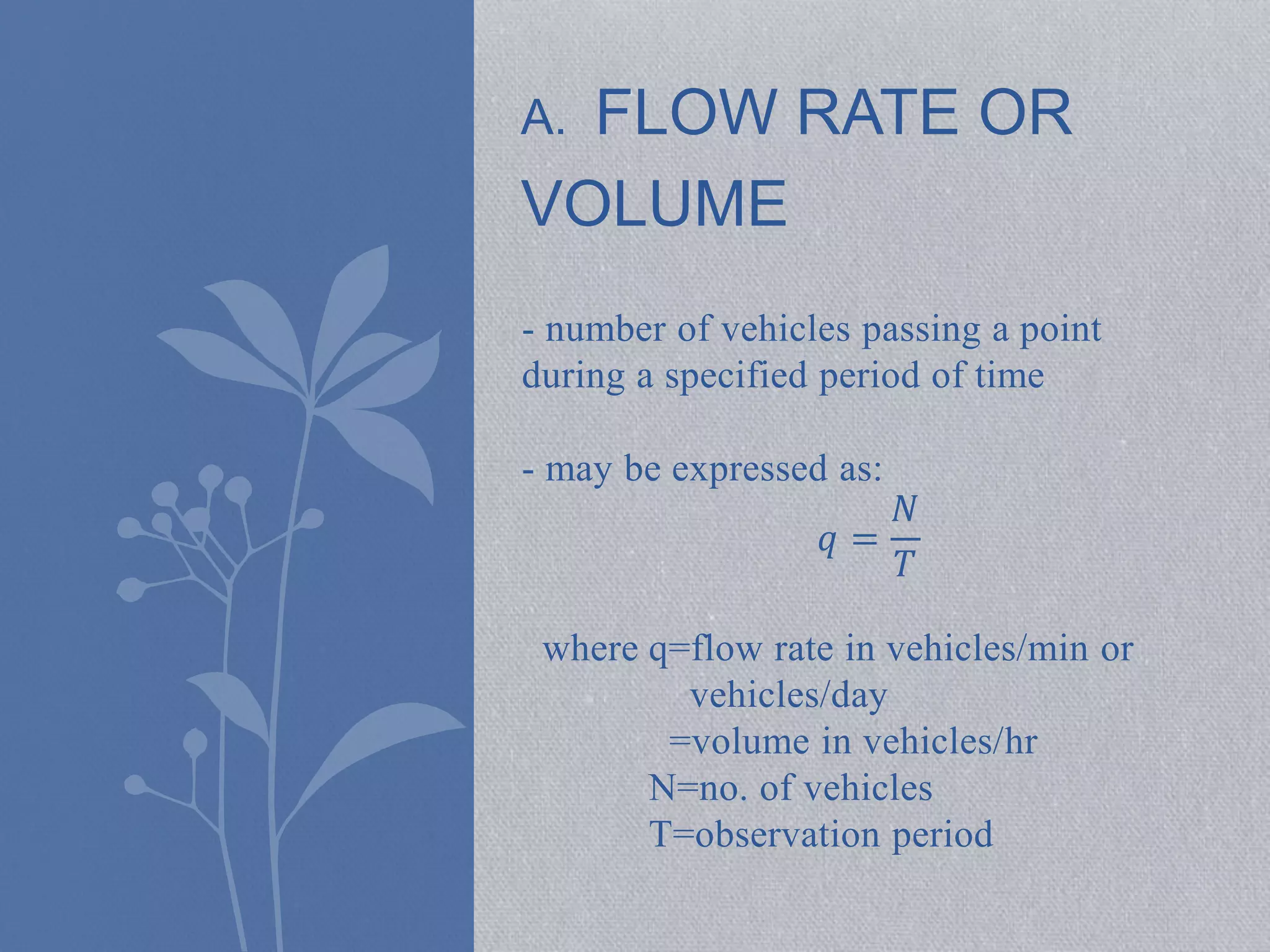
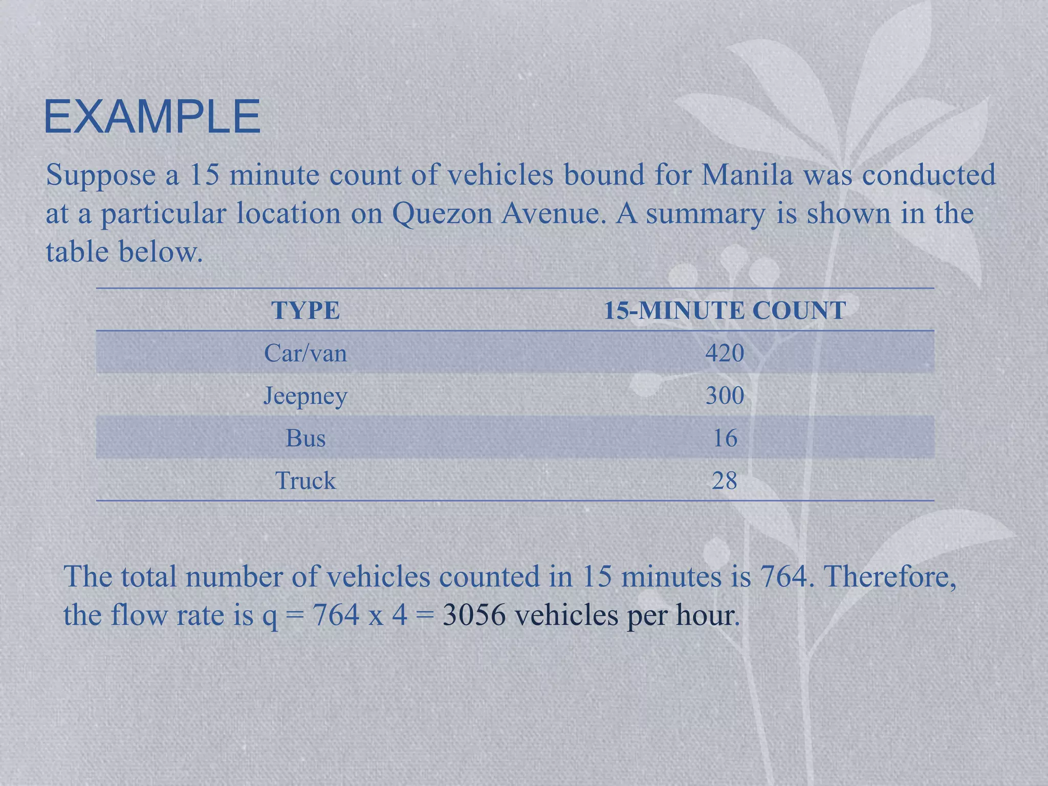
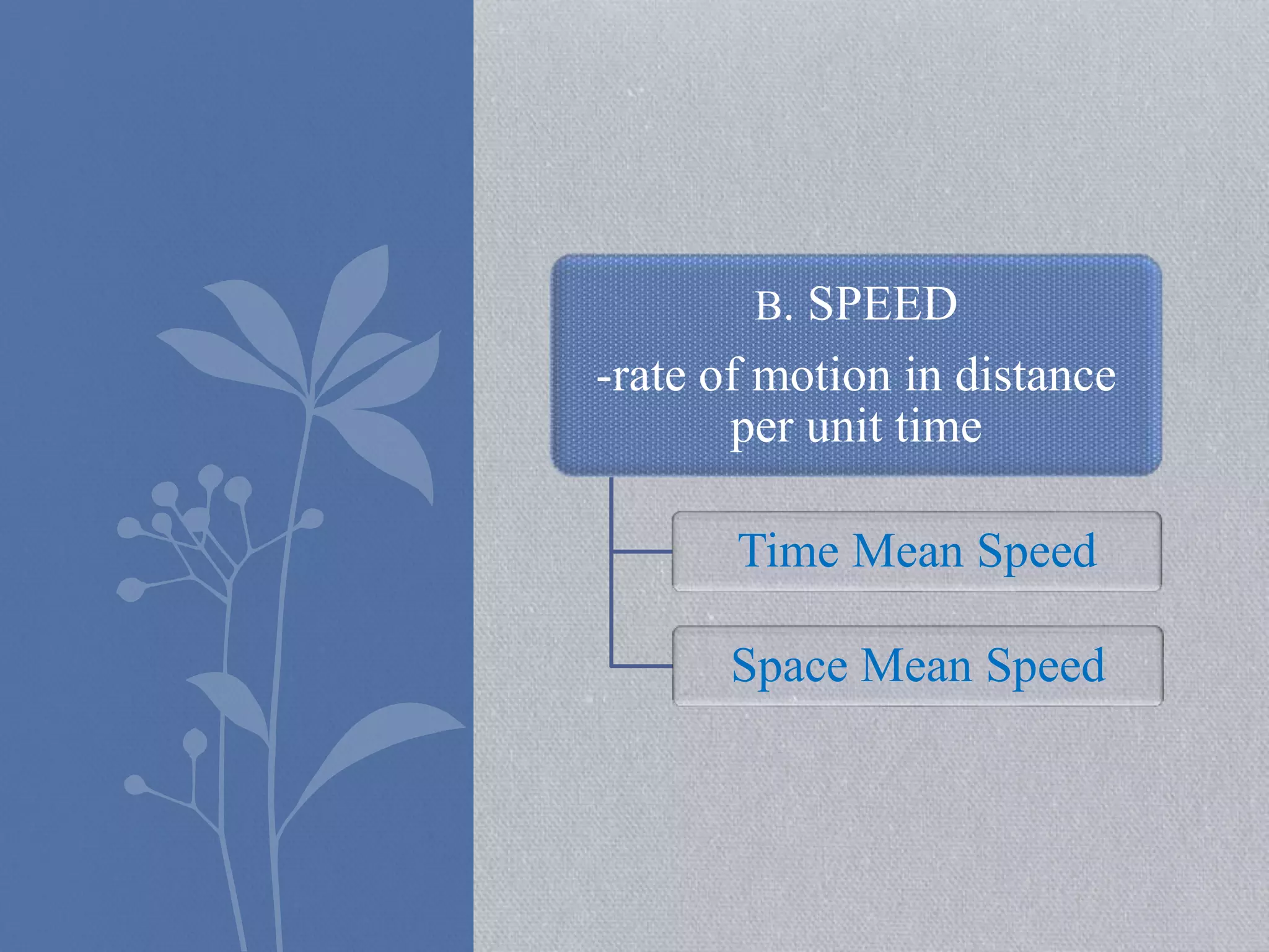
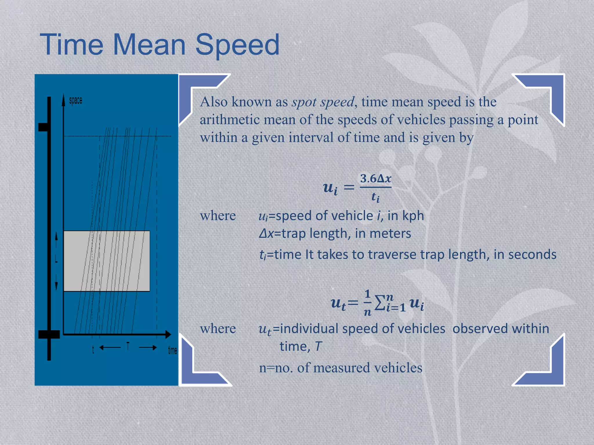
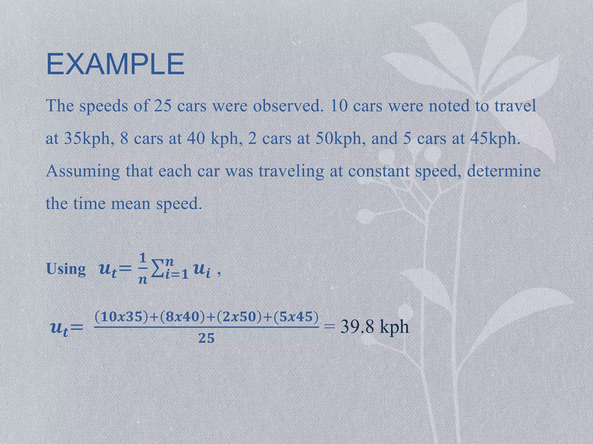
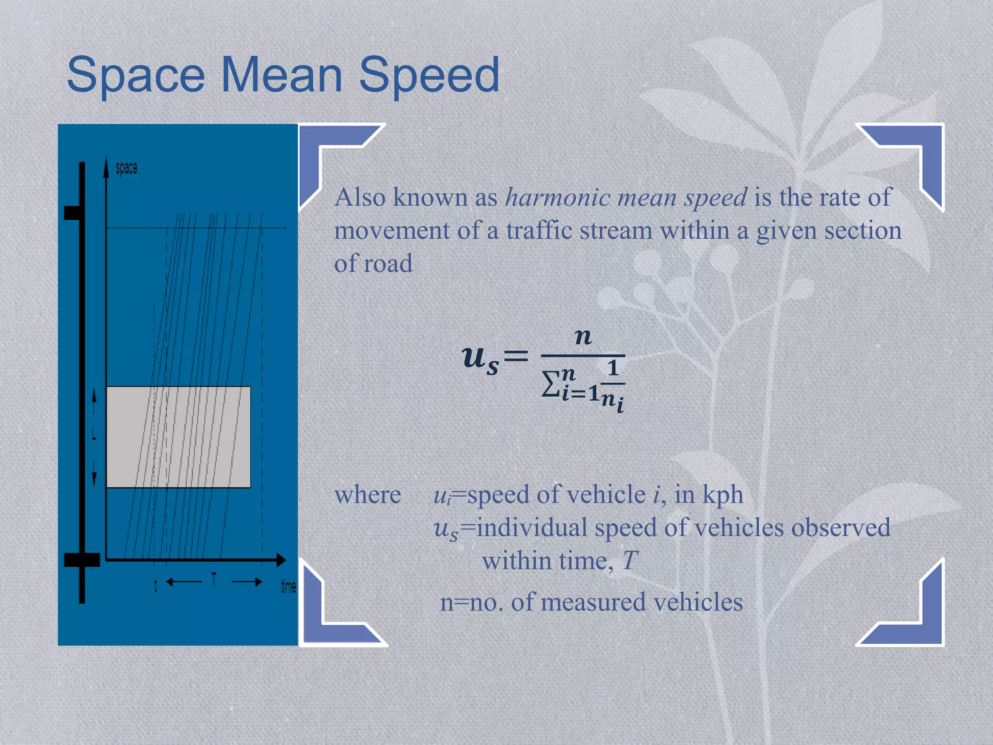
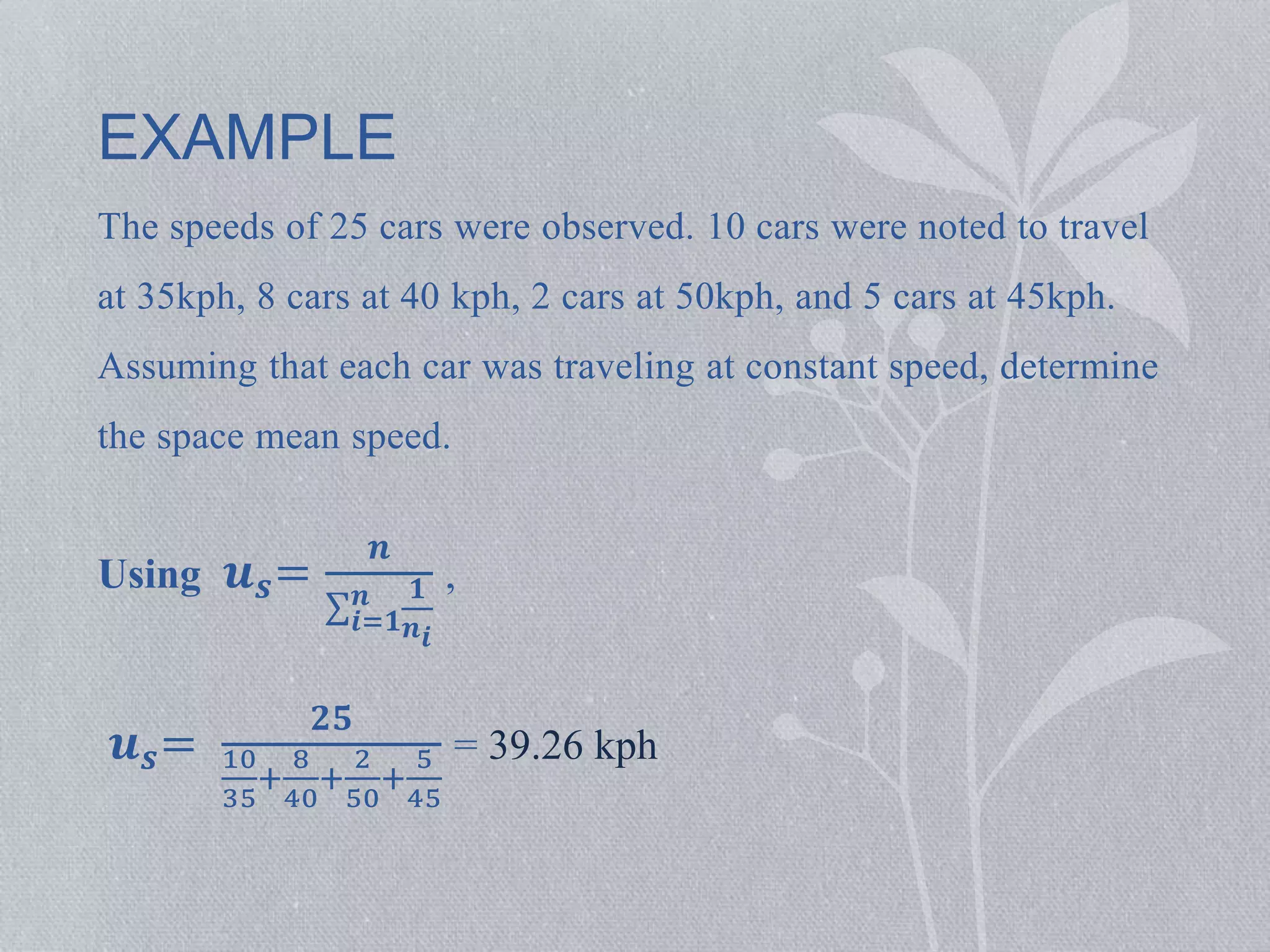
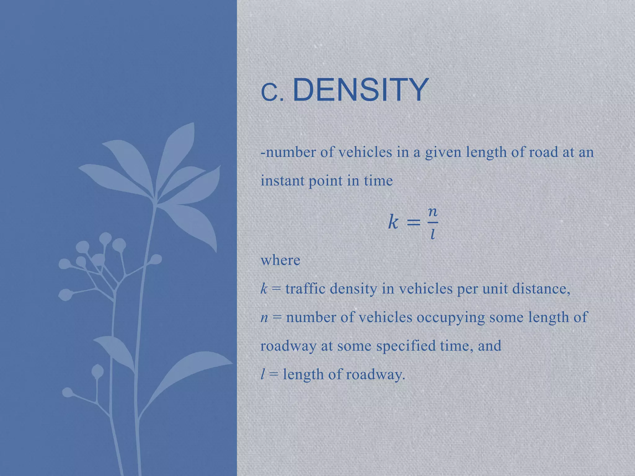
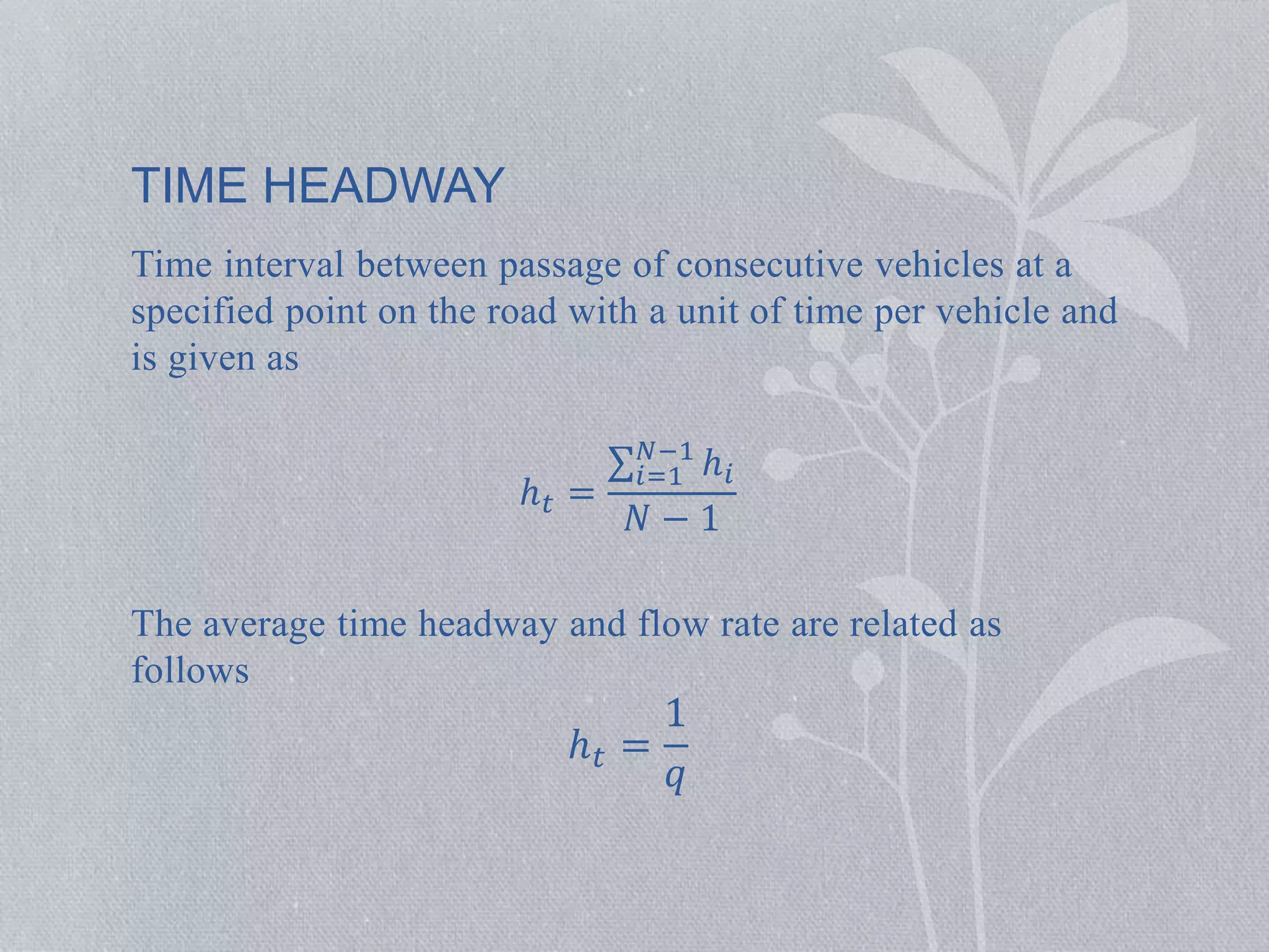
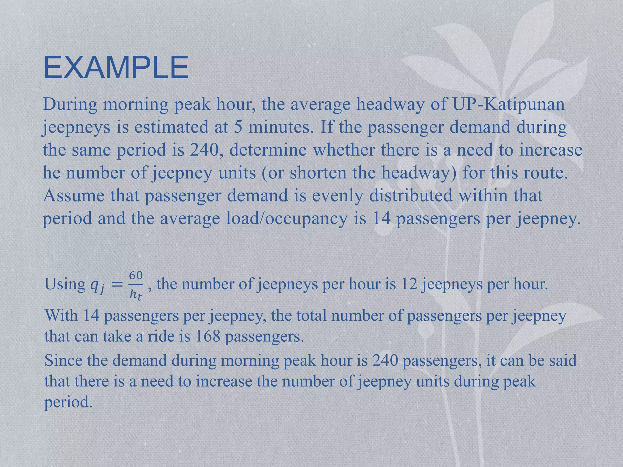
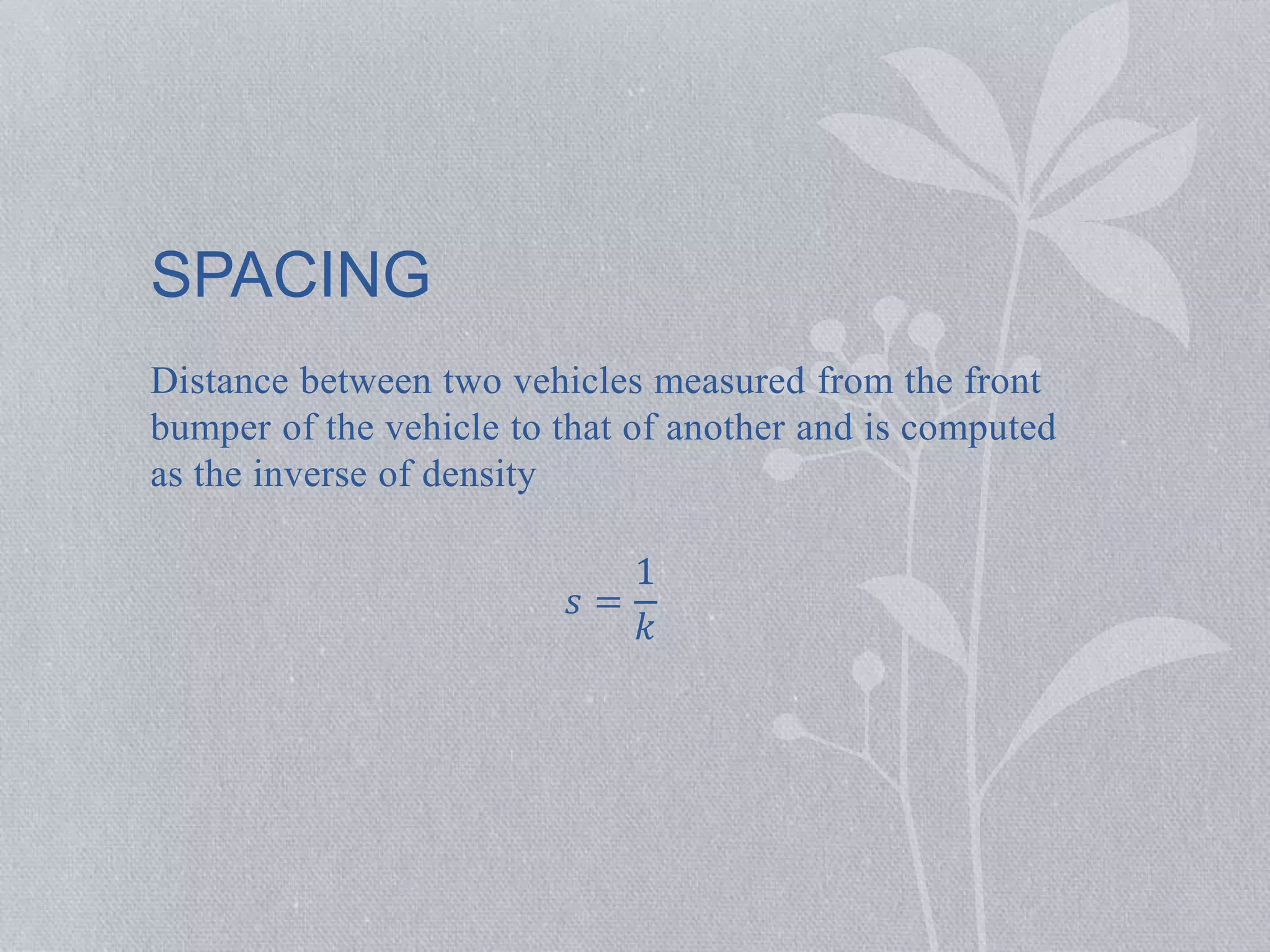
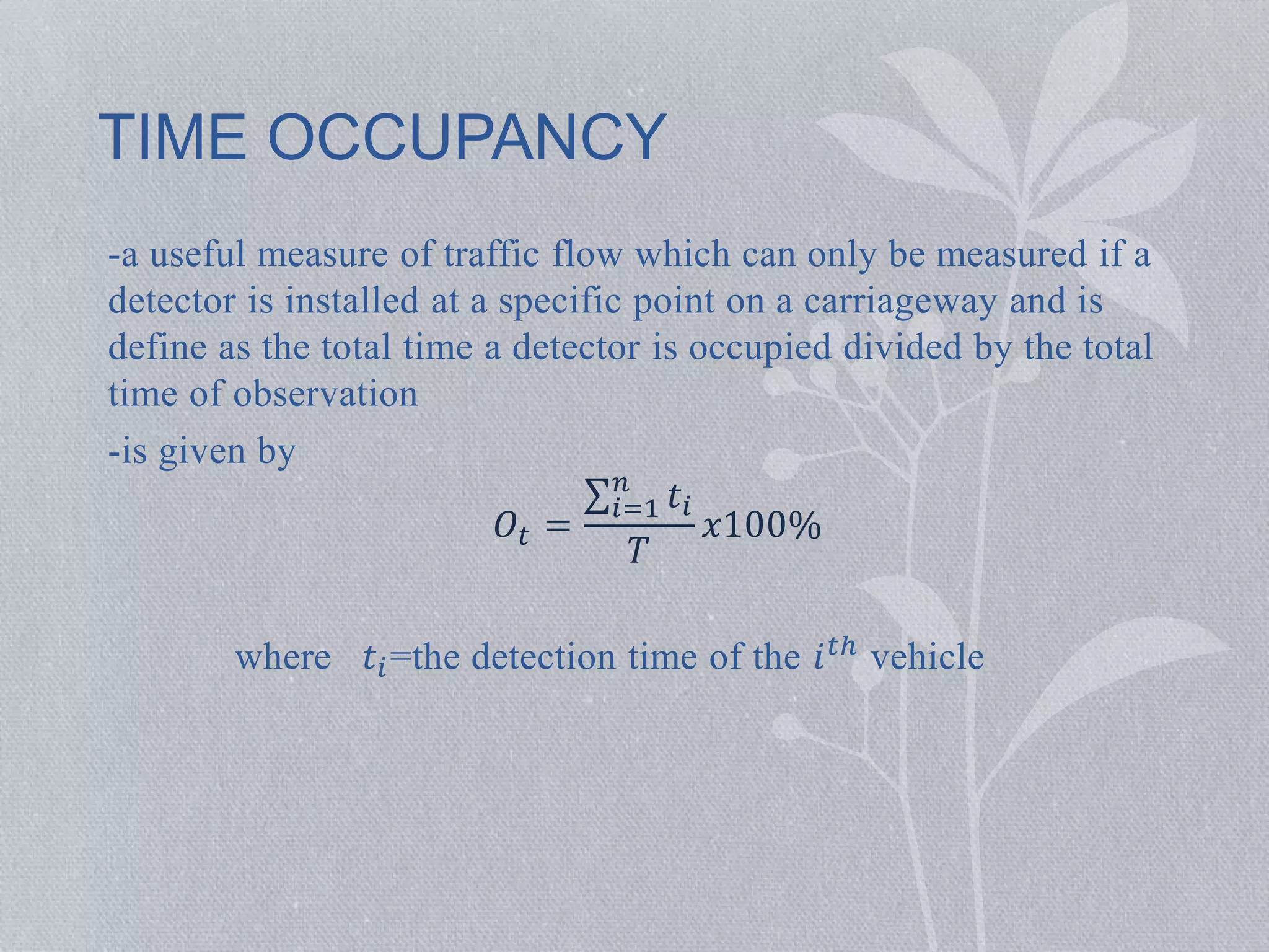
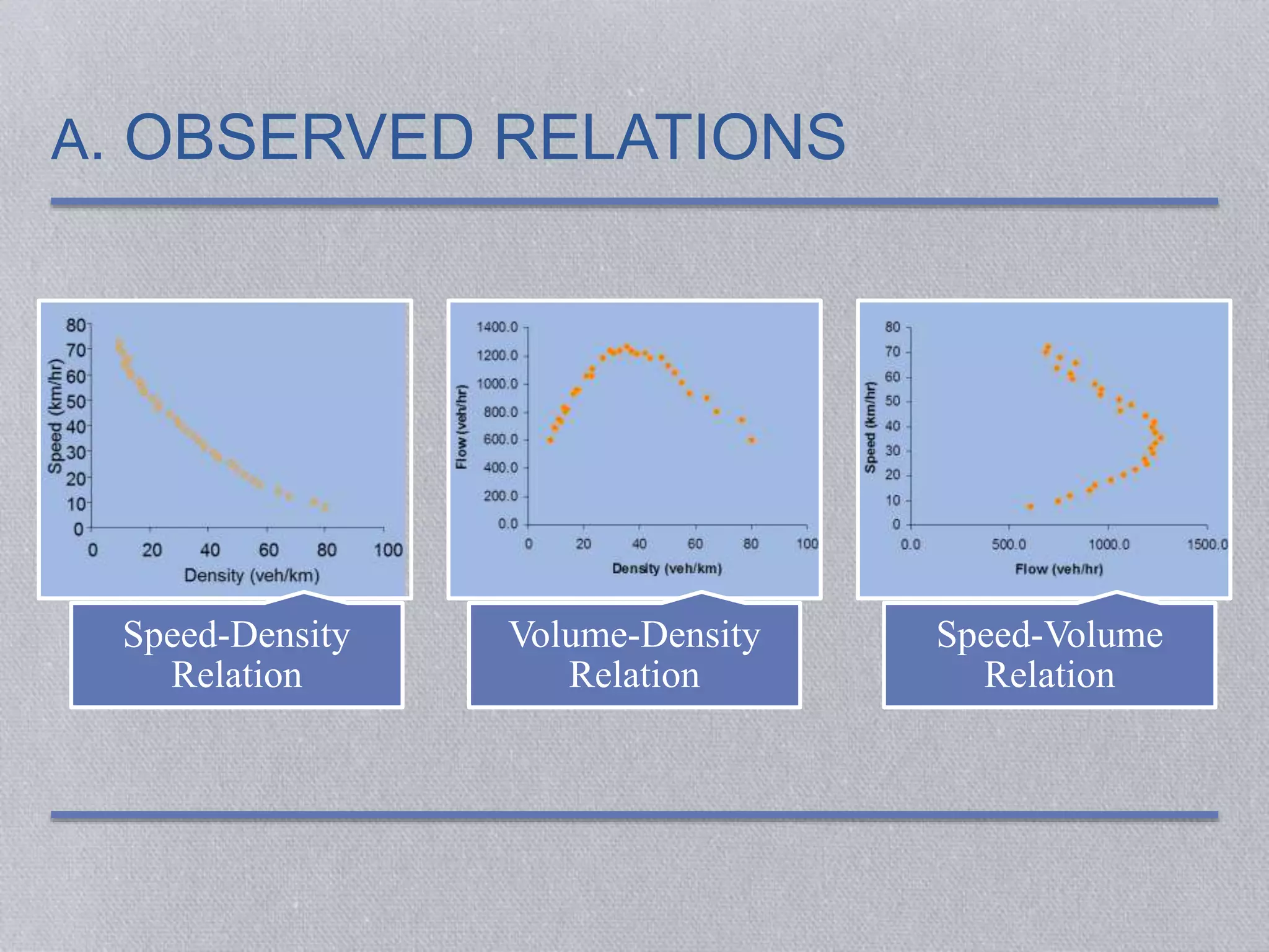
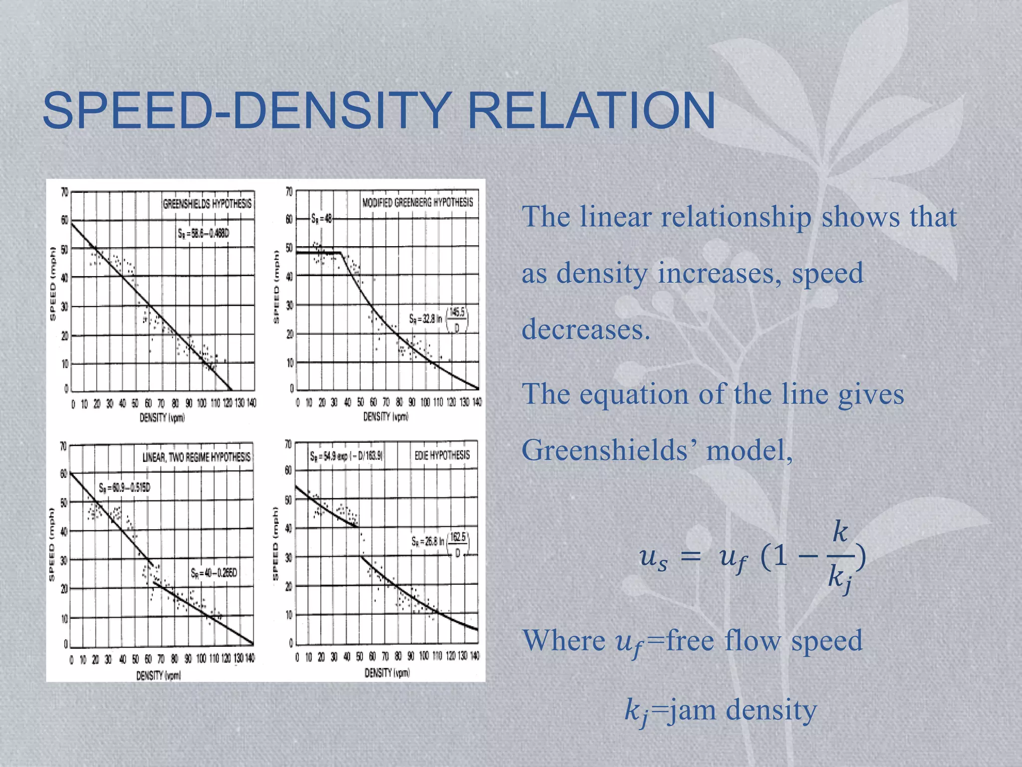
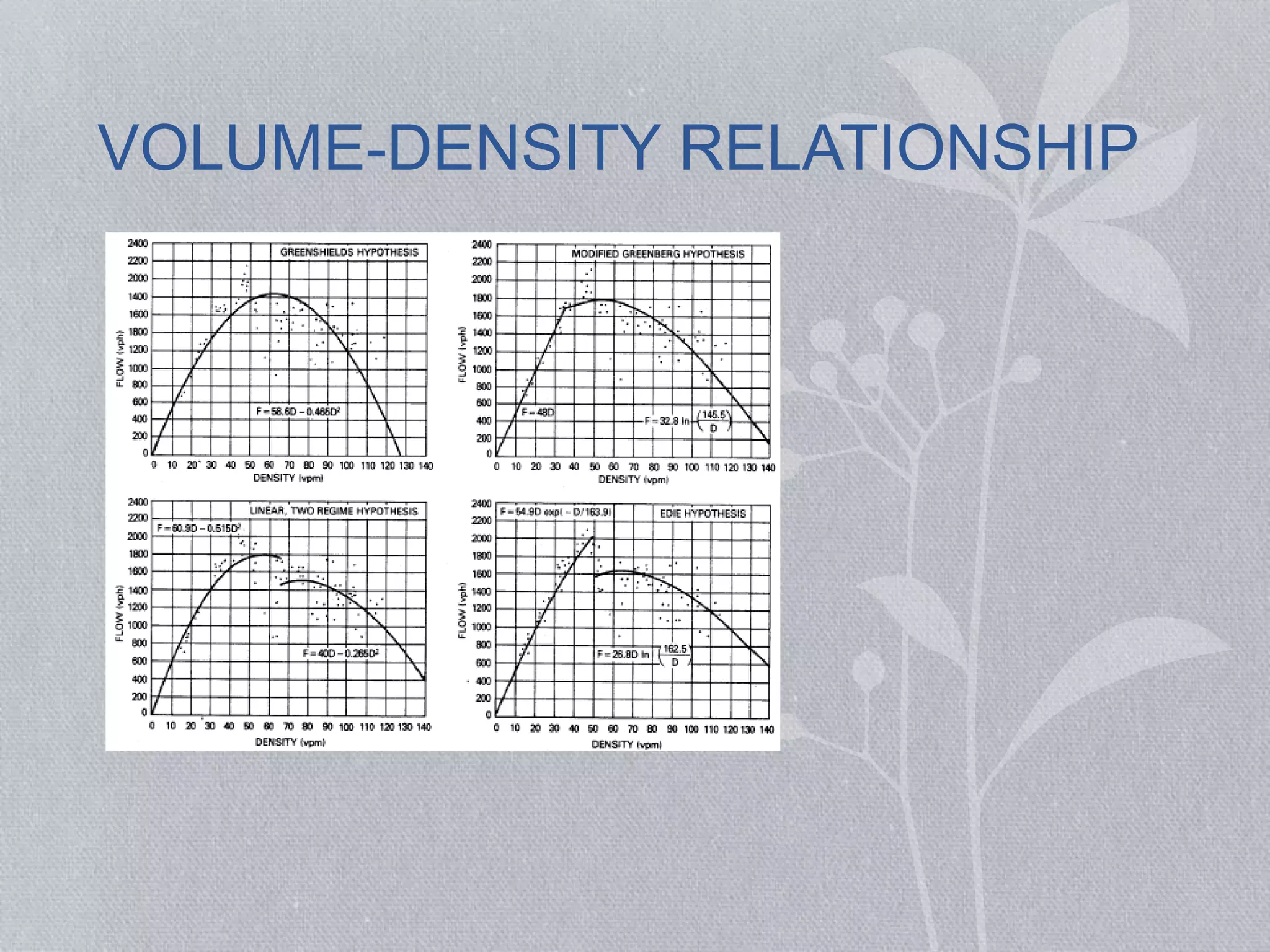
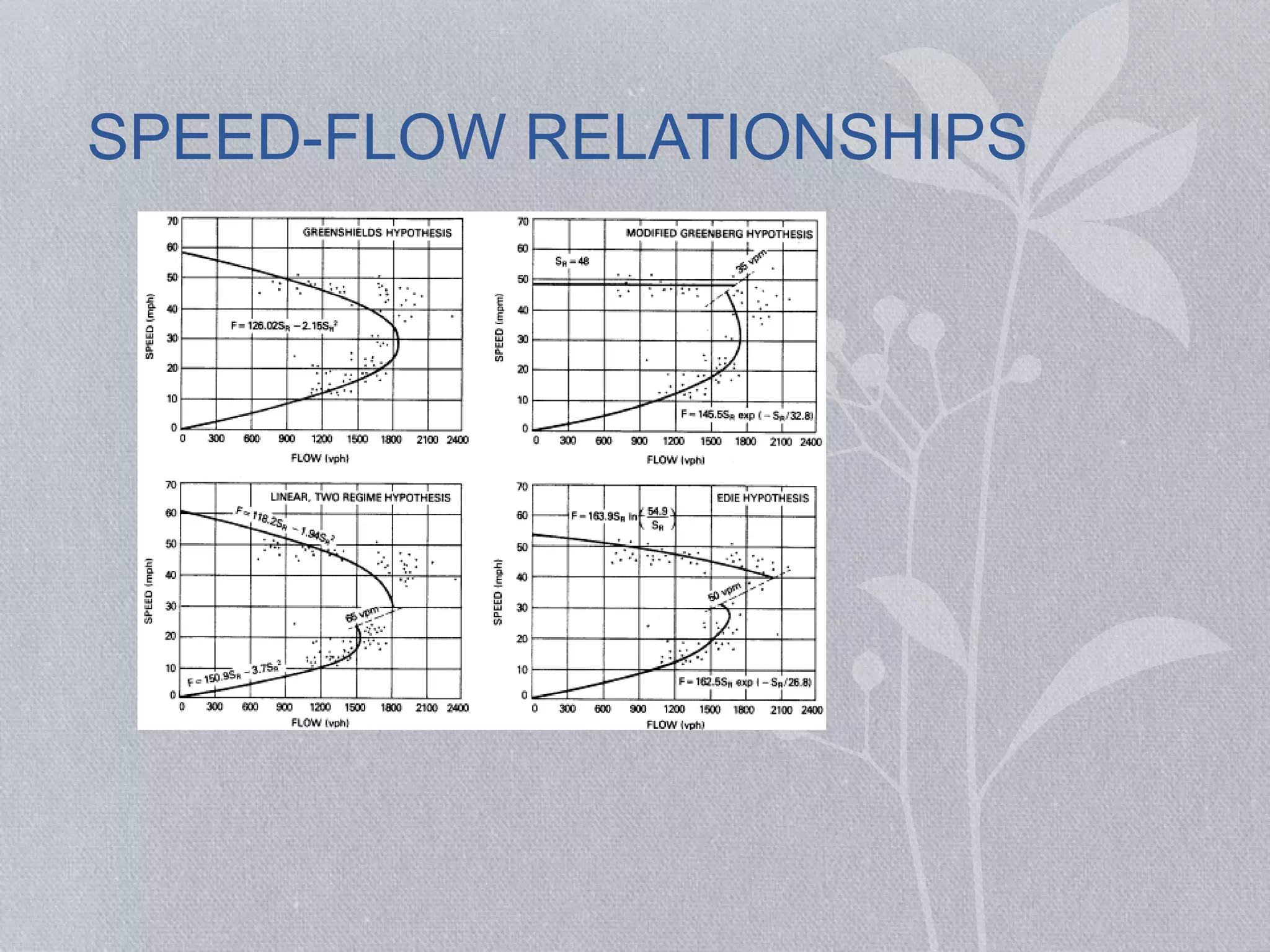
This document discusses traffic flow fundamentals, including different types of traffic flow and key variables used to describe traffic flow. It covers uninterrupted and interrupted flow, and variables such as flow rate, speed, density, time headway, spacing, and time occupancy. Empirical relationships between flow, speed, and density are presented, including the Greenshields speed-density model and equations relating volume to density. Examples are provided to demonstrate calculations for various traffic flow measures.

1. Traffic Flow Fundamentals
Introduction

2. TYPES OF FLOW
Traffic flow is usually classified as
either
a. Uninterrupted Flow
b. Interrupted Flow

3. A. UNINTERRUPTED FLOW
- flow occurring at long sections of
road where vehicles are not
required to stop by any cause
external to the traffic stream

4. B. INTERRUPTED FLOW
-flow occurring at long sections of road
where vehicles are required to stop by
any cause outside the traffic stream
such as traffic signs, traffic signal lights

5. UNINTERRUPTED
FLOW
Uninterrupted Flow can be described
using any of the following traffic
variables:
a. Flow rate or volume
b. Speed
c. Density or Concentration

6. A. FLOW RATE OR
VOLUME
- number of vehicles passing a point
during a specified period of time
- may be expressed as:
푞 =
푁
푇
where q=flow rate in vehicles/min or
vehicles/day
=volume in vehicles/hr
N=no. of vehicles
T=observation period

7. EXAMPLE
Suppose a 15 minute count of vehicles bound for Manila was conducted
at a particular location on Quezon Avenue. A summary is shown in the
table below.
TYPE 15-MINUTE COUNT
Car/van 420
Jeepney 300
Bus 16
Truck 28
The total number of vehicles counted in 15 minutes is 764. Therefore,
the flow rate is q = 764 x 4 = 3056 vehicles per hour.

8. B. SPEED
-rate of motion in distance
per unit time
Time Mean Speed
Space Mean Speed

9. Time Mean Speed
Also known as spot speed, time mean speed is the
arithmetic mean of the speeds of vehicles passing a point
within a given interval of time and is given by
풖풊 =
ퟑ.ퟔ횫풙
풕풊
where uᵢ=speed of vehicle i, in kph
Δx=trap length, in meters
tᵢ=time It takes to traverse trap length, in seconds
풖풕=
ퟏ
풏
풏 풖풊
풊=ퟏ
where 푢푡=individual speed of vehicles observed within
time, T
n=no. of measured vehicles

10. EXAMPLE
The speeds of 25 cars were observed. 10 cars were noted to travel
at 35kph, 8 cars at 40 kph, 2 cars at 50kph, and 5 cars at 45kph.
Assuming that each car was traveling at constant speed, determine
the time mean speed.
Using 풖풕=
ퟏ
풏
풏 풖풊 ,
풊=ퟏ
풖풕=
ퟏퟎ풙ퟑퟓ + ퟖ풙ퟒퟎ + ퟐ풙ퟓퟎ +(ퟓ풙ퟒퟓ)
ퟐퟓ
= 39.8 kph

11. Space Mean Speed
Also known as harmonic mean speed is the rate of
movement of a traffic stream within a given section
of road
풖풔=
풏
풏 ퟏ
풊=ퟏ
풏풊
where uᵢ=speed of vehicle i, in kph
푢푠=individual speed of vehicles observed
within time, T
n=no. of measured vehicles

12. EXAMPLE
The speeds of 25 cars were observed. 10 cars were noted to travel
at 35kph, 8 cars at 40 kph, 2 cars at 50kph, and 5 cars at 45kph.
Assuming that each car was traveling at constant speed, determine
the space mean speed.
Using 풖풔=
풏
풏 ퟏ
풊=ퟏ
풏풊
,
풖풔=
ퟐퟓ
10
35
+
8
40
+
2
50
+
5
45
= 39.26 kph

13. C. DENSITY
-number of vehicles in a given length of road at an
instant point in time
푘 =
푛
푙
where
k = traffic density in vehicles per unit distance,
n = number of vehicles occupying some length of
roadway at some specified time, and
l = length of roadway.

14. OTHER TRAFFIC
VARIABLES
Other variables used to described traffic
flow are simply variants of the previous
variables.
a. Time Headway
b. Spacing
c. Time Occupancy

15. Time interval between passage of consecutive vehicles at a
specified point on the road with a unit of time per vehicle and
is given as
ℎ푡 =
푁−1 푖=1
ℎ푖
푁 − 1
The average time headway and flow rate are related as
follows
ℎ푡 =
1
푞
TIME HEADWAY

16. EXAMPLE
During morning peak hour, the average headway of UP-Katipunan
jeepneys is estimated at 5 minutes. If the passenger demand during
the same period is 240, determine whether there is a need to increase
he number of jeepney units (or shorten the headway) for this route.
Assume that passenger demand is evenly distributed within that
period and the average load/occupancy is 14 passengers per jeepney.
Using 푞푗 =
60
ℎ푡
, the number of jeepneys per hour is 12 jeepneys per hour.
With 14 passengers per jeepney, the total number of passengers per jeepney
that can take a ride is 168 passengers.
Since the demand during morning peak hour is 240 passengers, it can be said
that there is a need to increase the number of jeepney units during peak
period.

17. SPACING
Distance between two vehicles measured from the front
bumper of the vehicle to that of another and is computed
as the inverse of density
푠 =
1
푘

18. EXAMPLE
During heavy traffic congestion, it was observed that the average
spacing of vehicles in queue in the innermost lane in EDSA is 6.5m.
Determine the jam density or density of stopped vehicles.
Using 푠 =
1
푘
,
The jam density is 푘푗 =
1000
6.5
= 153.85 vehicles/km

19. TIME OCCUPANCY
-a useful measure of traffic flow which can only be measured if a
detector is installed at a specific point on a carriageway and is
define as the total time a detector is occupied divided by the total
time of observation
-is given by
푂푡 =
푛 푖=1
푡푖
푇
푥100%
where 푡푖=the detection time of the 푖푡ℎ vehicle

20. RELATIONSHIP OF
FLOW, SPEED AND
DENSITY
A relationship exists among the three most
important traffic variables: flow rate, space
mean speed and density.
a. Observed Relations
b. Empirical Relations

21. A. OBSERVED RELATIONS
Speed-Density
Relation
Volume-Density
Relation
Speed-Volume
Relation

22. B. EMPIRICAL
RELATIONS
Speed-density relation
Volume-density relation
Volume-speed relation

23. SPEED-DENSITY RELATION
The linear relationship shows that
as density increases, speed
decreases.
The equation of the line gives
Greenshields’ model,
푢푠 = 푢푓 (1 −
푘
푘푗
)
Where 푢푓=free flow speed
푘푗=jam density

24. VOLUME-DENSITY RELATIONSHIP

25. SPEED-FLOW RELATIONSHIPS