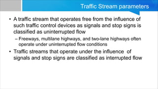
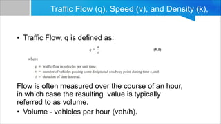
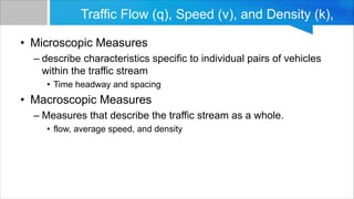
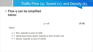
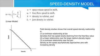
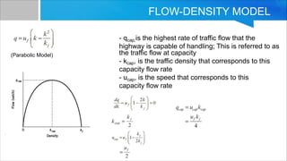
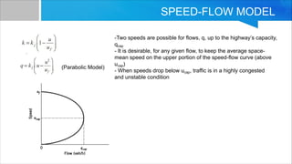
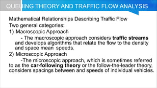
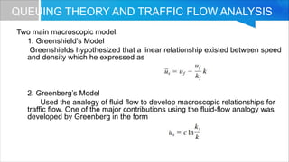
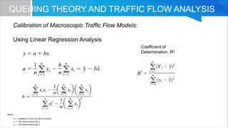
This document discusses fundamentals of traffic flow and queuing theory. It defines traffic flow parameters for uninterrupted and interrupted traffic streams. It describes traffic flow, speed, and density measurements including volume, time headway, average and space mean speed, and density. It presents speed-density, flow-density, and speed-flow models and discusses macroscopic and microscopic traffic flow approaches. It also introduces Greenshields and Greenberg traffic flow models and how to calibrate macroscopic models using linear regression analysis.

1. Fundamentals of Traffic Flow and Queuing
Theory

2. Traffic Stream parameters
• A traffic stream that operates free from the influence of
such traffic control devices as signals and stop signs is
classified as uninterrupted flow
– Freeways, multilane highways, and two-lane highways often
operate under uninterrupted flow conditions
• Traffic streams that operate under the influence of
signals and stop signs are classified as interrupted flow

3. Traffic Flow (q), Speed (v), and Density (k),
• Traffic Flow, q is defined as:
Flow is often measured over the course of an hour,
in which case the resulting value is typically
referred to as volume.
• Volume - vehicles per hour (veh/h).

4. Traffic Flow (q), Speed (v), and Density (k),
• The time between the passage of the front
bumpers of successive vehicles, at some
designated highway point, is known as the time
headway.

5. Traffic Flow (q), Speed (v), and Density (k),

6. Traffic Flow (q), Speed (v), and Density (k),
• Average Traffic Speed
– Time Mean Speed

7. Traffic Flow (q), Speed (v), and Density (k),
• Average Traffic Speed
– Space Mean Speed (Harmonic Mean Speed)

8. Traffic Flow (q), Speed (v), and Density (k),
• Density
– The density can also be related to the individual
spacing between successive vehicles (measured
from front bumper to front bumper).

9. Traffic Flow (q), Speed (v), and Density (k),
• Density

10. Traffic Flow (q), Speed (v), and Density (k),
• Microscopic Measures
– describe characteristics specific to individual pairs of vehicles
within the traffic stream
• Time headway and spacing
• Macroscopic Measures
– Measures that describe the traffic stream as a whole.
• flow, average speed, and density

11. Traffic Flow (q), Speed (v), and Density (k),
• Flow q can be simplified
below:

12. Sample problem 1

13. Sample problem 2

14. Sample problem 3
Problem 3: Determining Flow, Density, Time Mean Speed, and Space Mean Speed
The figure shows vehicles traveling at constant speeds on a two-lane highway between sections X and Y with their positions and
speeds obtained at an instant of time by photography. An observer located at point X observes the four vehicles passing point X
during a period of T sec. The velocities of the vehicles are measured as 45, 45, 40, and 30 mi/h, respectively. Calculate the flow,
density, time mean speed, and space mean speed.
�����: � = 4, �� = 45��/ℎ, �� = 45��/ℎ,
�� = 40��/ℎ, �� = 30��/ℎ
Solving for flow q,
� =
�
�
� 3600 =
4�3600
�
=
��,���
�
���/�
Solving for density k,
� =
�
�
� 5280 =
4�5280
300
= ��. ����/��
Solving for time mean speed ��,
�� =
45+45+40+30
4
= 40��/ℎ
Solving for space mean speed ��,
�� =
��
�1+�2+�3+�4
Solving for space mean speed ��,
�� =
��
�1+�2+�3+�4
�� =
��
��
�� =
300��
45��/ℎ�(
5280��
1��
)(
1ℎ�
3600���
)
= 4.545����
�� =
300��
45��/ℎ�(
5280��
1��
)(
1ℎ�
3600���
)
= 4.545����
�� =
300��
40��/ℎ�(
5280��
1��
)(
1ℎ�
3600���
)
= 5.114����
�� =
300��
30��/ℎ�(
5280��
1��
)(
1ℎ�
3600���
)
= 6.818����
Solving for space mean speed ��,
�� =
4�300
4.545+4.545+5.114+6.818
�� = 57.083��/���
�� = 38.920��/ℎ�

15. BASIC TRAFFIC STREAM MODELS
These models will help us understand the interaction of
the individual macroscopic measures in order to fully
analyze the operational performance of traffic streams

16. SPEED-DENSITY MODEL
a. For Very Low density highway, driver will be able to travel freely at a
speed close to the design speed of the highway.
b. As more and more vehicles begin to use a section of highway, the traffic
density will increase and the average operating speed of vehicles will
decline from the free-flow value as drivers slow to allow for the maneuvers of
other vehicles.
c. Eventually, the highway section will become so congested (will have such
a high density) that the traffic will come to a stop (u = 0), and the density will
be determined by the length of the vehicles and the spaces that drivers
leave between them.

17. SPEED-DENSITY MODEL
Field density studies shows that overall speed-density realtionship
is:
(1) a nonlinear relationship at low
densities that has speed slowly declining from the free-flow value
(2) a linear relationship over the large medium-density region
(3) a nonlinear relationship near the jam
density as the speed asymptotically approaches zero with
increasing density
(Linear Model)

18. Solution to Problem 1

19. FLOW-DENSITY MODEL
- qcap,is the highest rate of traffic flow that the
highway is capable of handling; This is referred to as
the traffic flow at capacity
- kcap, is the traffic density that corresponds to this
capacity flow rate
- ucap, is the speed that corresponds to this
capacity flow rate
(Parabolic Model)

20. SPEED-FLOW MODEL
(Parabolic Model)
-Two speeds are possible for flows, q, up to the highway’s capacity,
qcap
- It is desirable, for any given flow, to keep the average space-
mean speed on the upper portion of the speed-flow curve (above
ucap)
- When speeds drop below ucap, traffic is in a highly congested
and unstable condition

21. Sample problem 4

22. QUEUING THEORY AND TRAFFIC FLOW ANALYSIS
Mathematical Relationships Describing Traffic Flow
Two general categories:
1) Macroscopic Approach
- The macroscopic approach considers traffic streams
and develops algorithms that relate the flow to the density
and space mean speeds.
2) Microscopic Approach
-The microscopic approach, which is sometimes referred
to as the car-following theory or the follow-the-leader theory,
considers spacings between and speeds of individual vehicles.

23. QUEUING THEORY AND TRAFFIC FLOW ANALYSIS
Two main macroscopic model:
1. Greenshield’s Model
Greenshields hypothesized that a linear relationship existed between speed
and density which he expressed as
2. Greenberg’s Model
Used the analogy of fluid flow to develop macroscopic relationships for
traffic flow. One of the major contributions using the fluid-flow analogy was
developed by Greenberg in the form

24. QUEUING THEORY AND TRAFFIC FLOW ANALYSIS
Calibration of Macroscopic Traffic Flow Models:
Using Linear Regression Analysis
Coefficient of
Determination, R2

25. Sample Problem 5
Use Linear Regression Analysis to solve ��, ��,
equation of ��, and R²