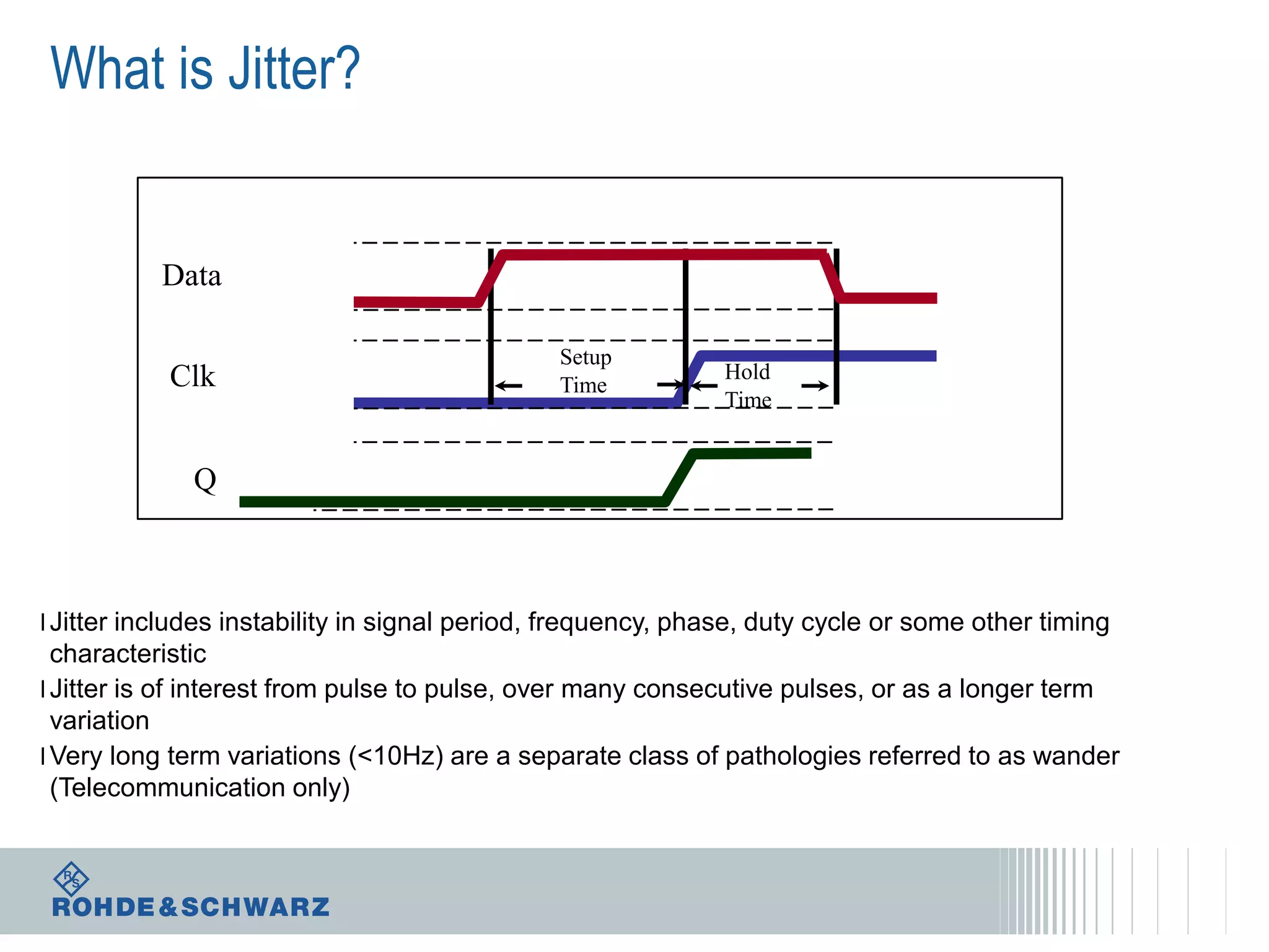
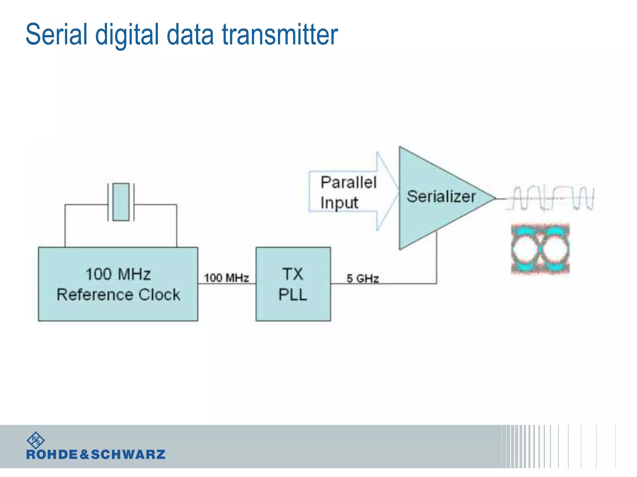
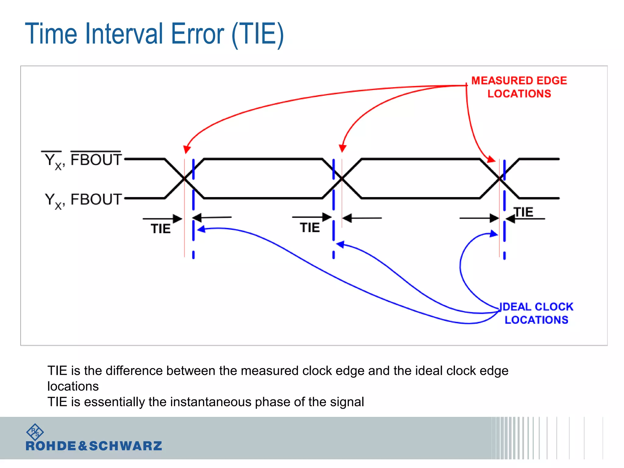
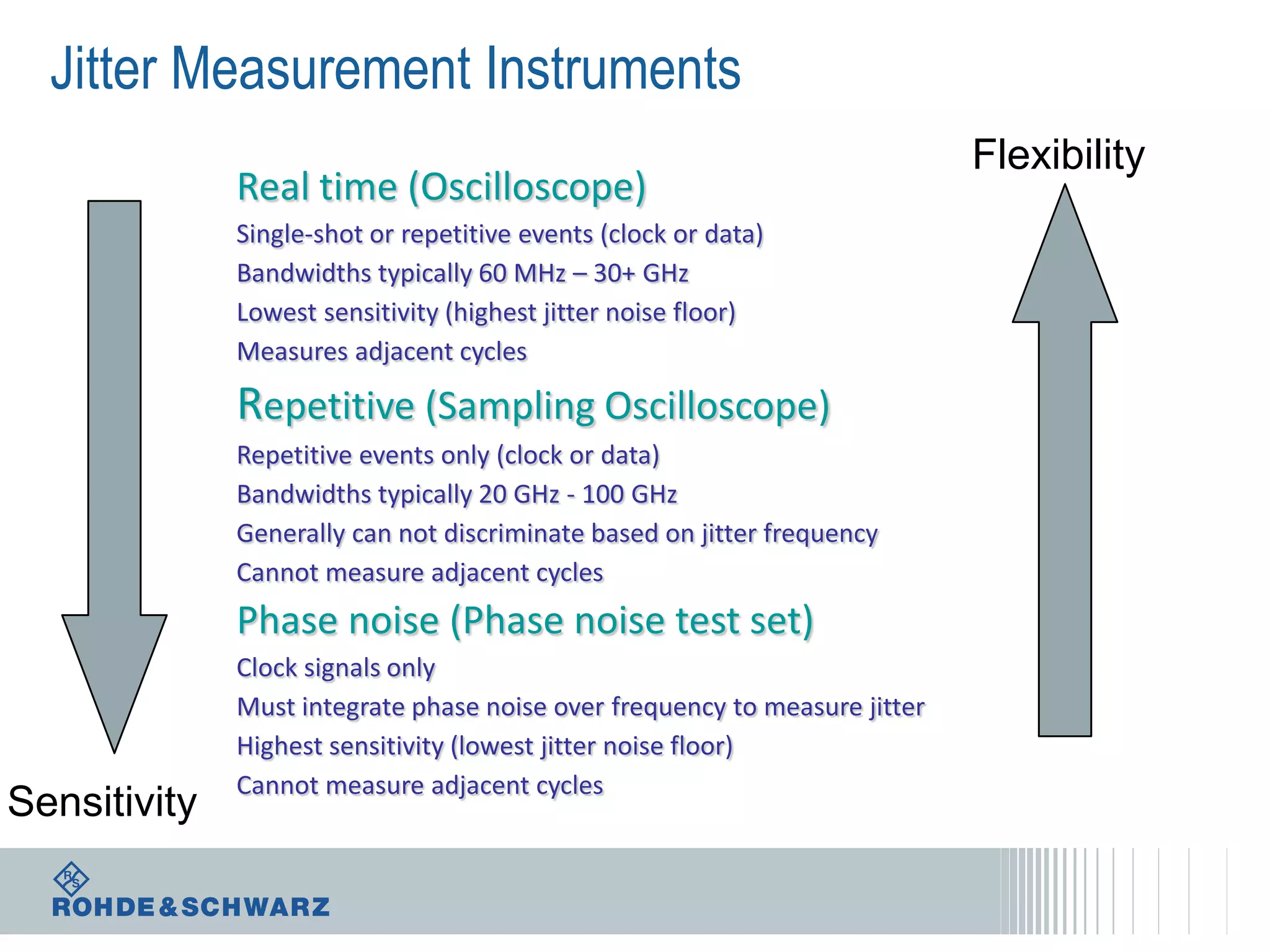
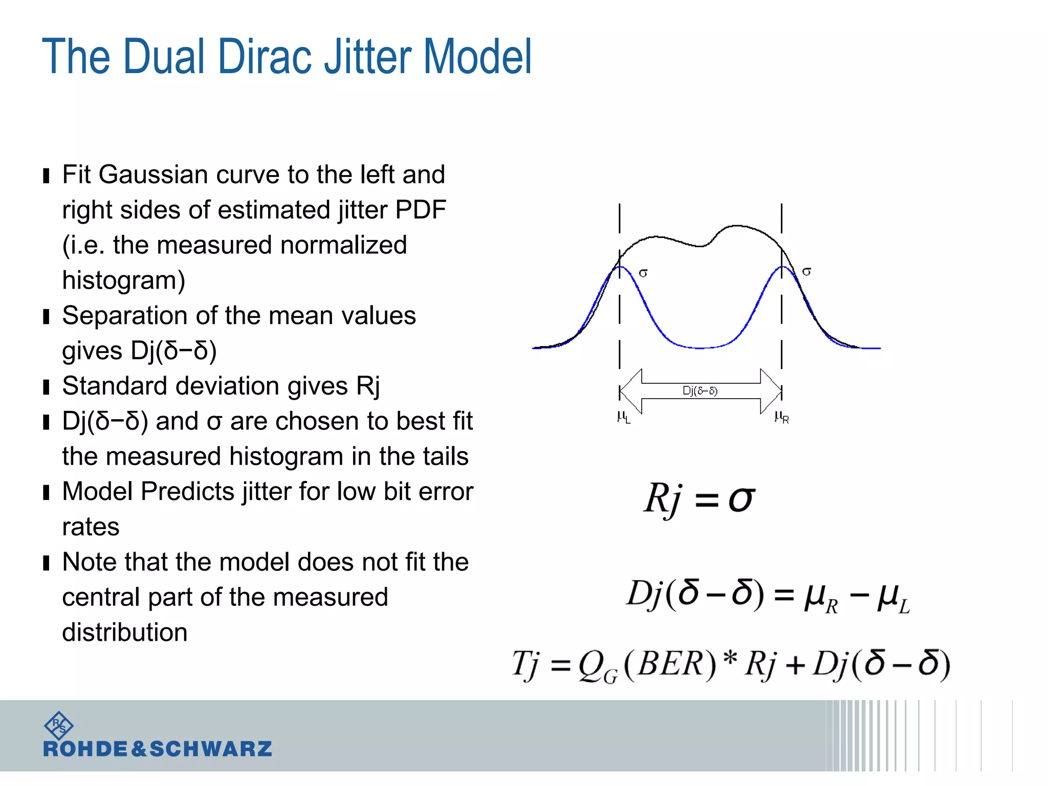
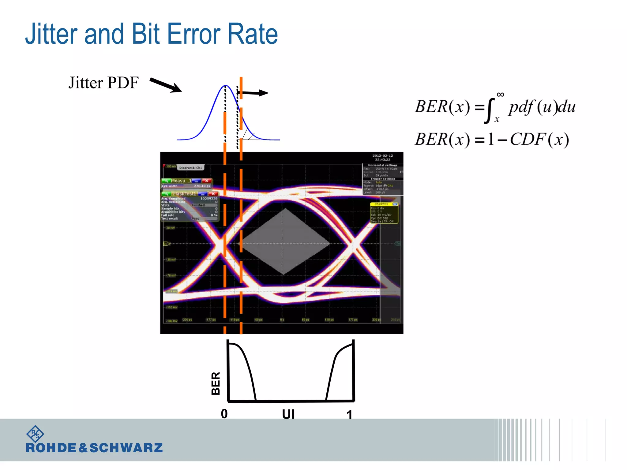
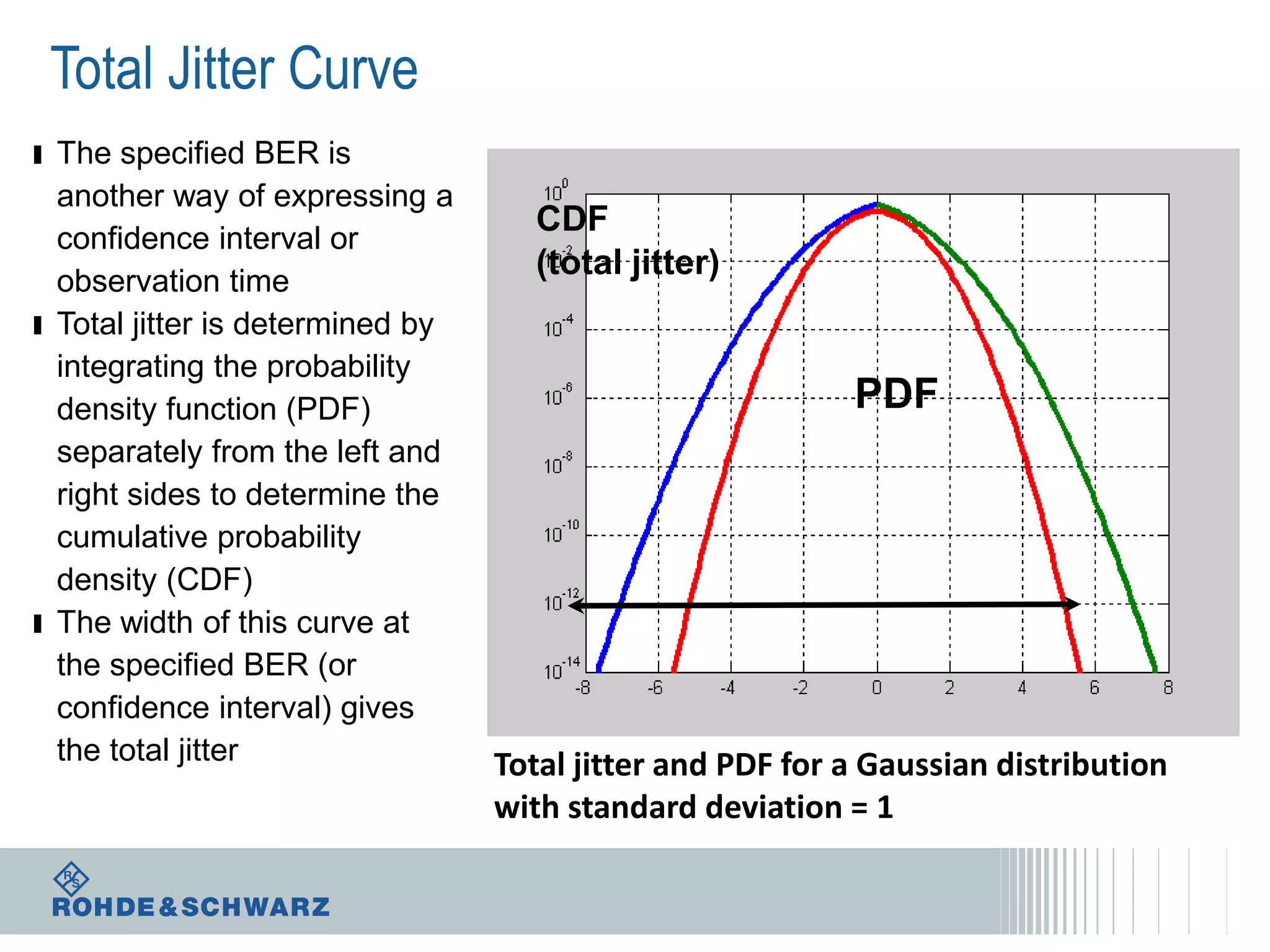
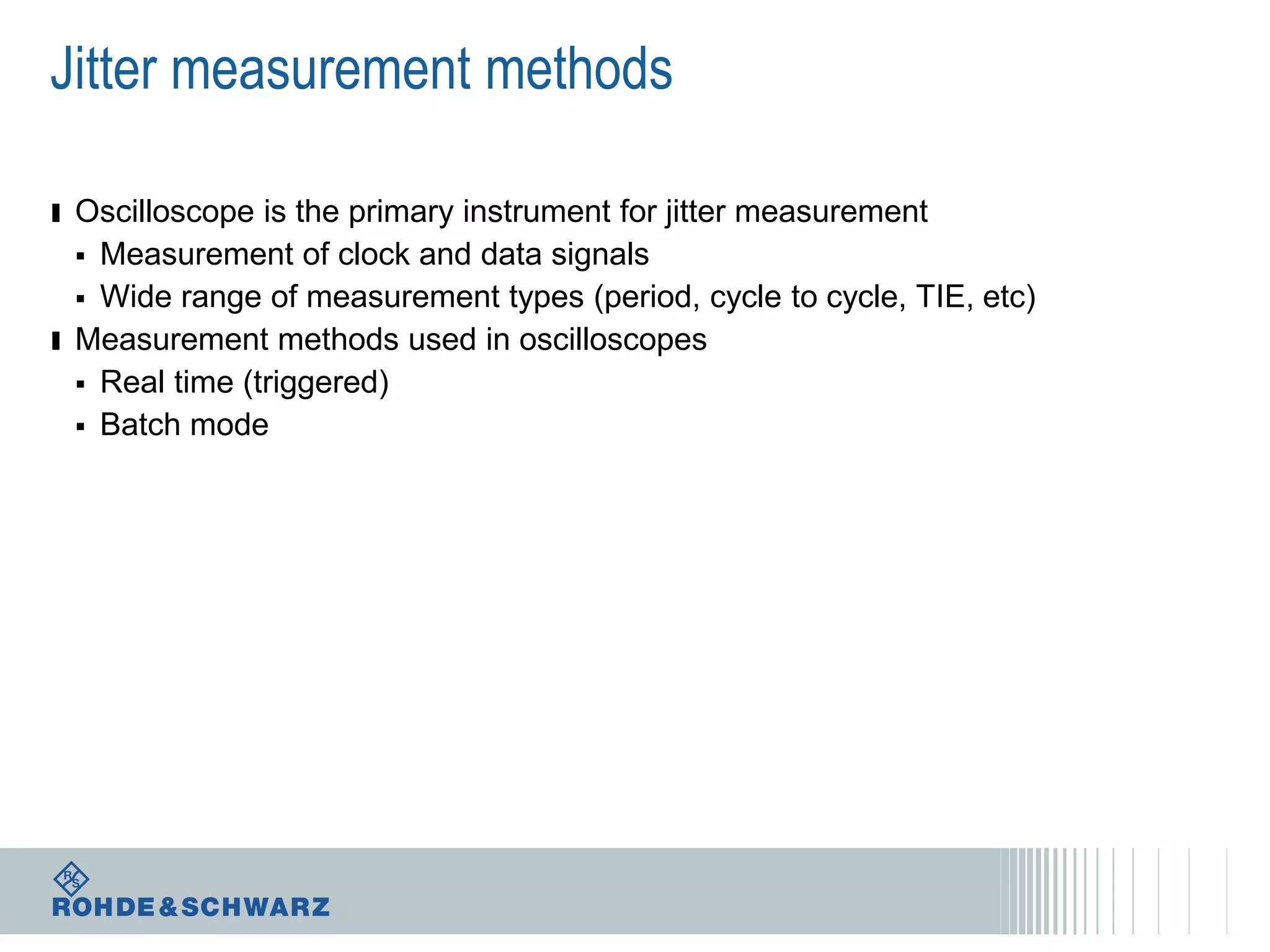
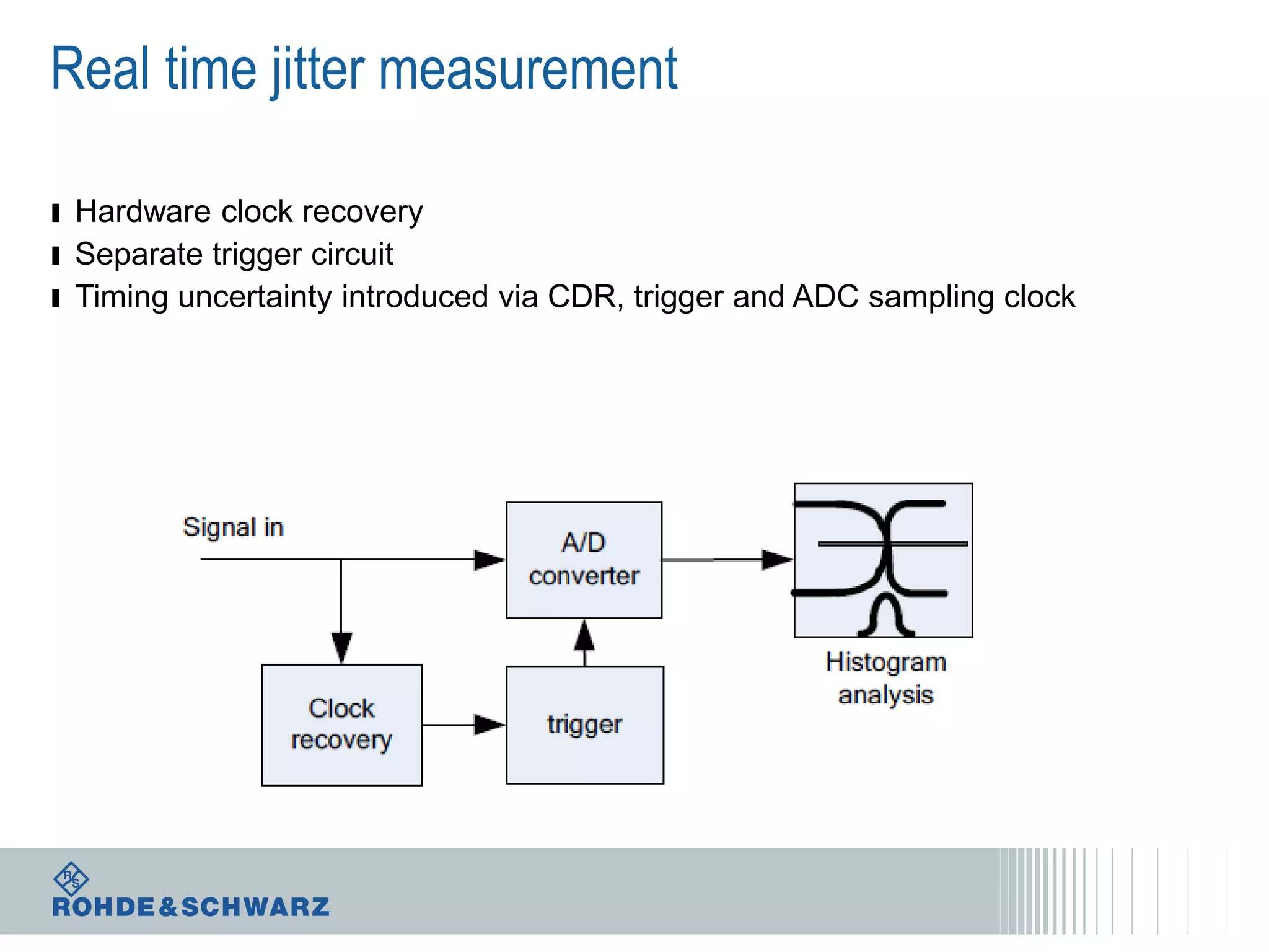
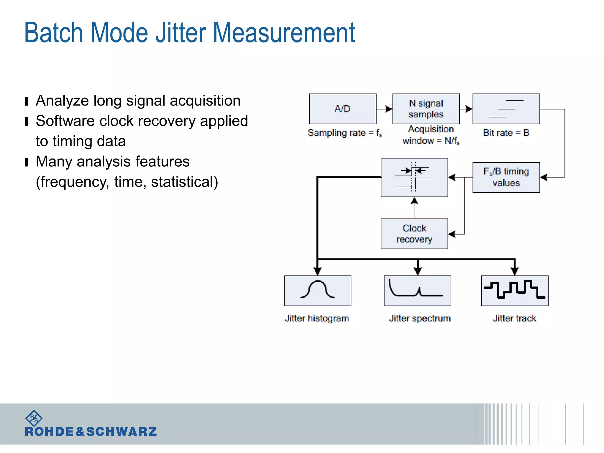
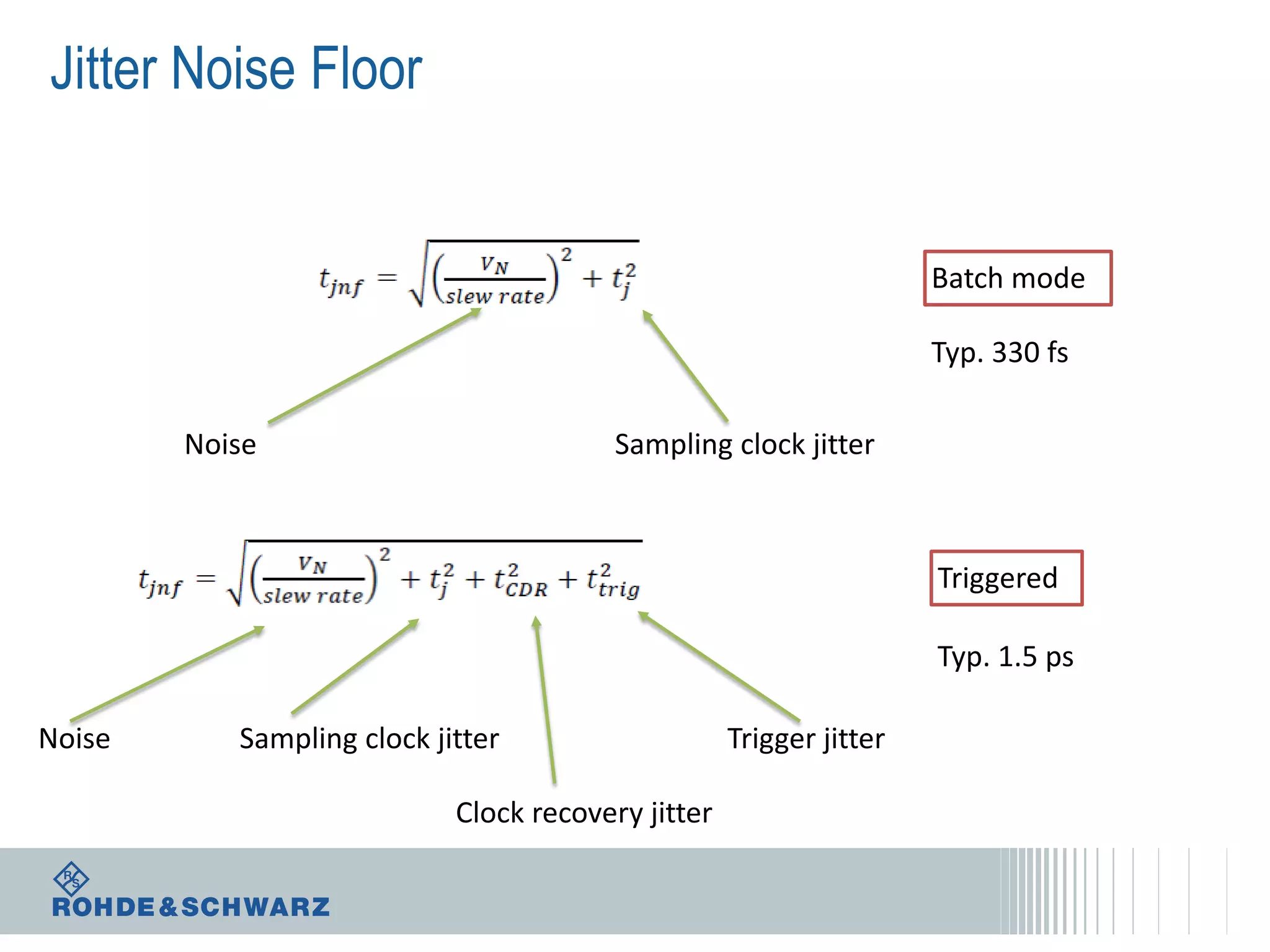
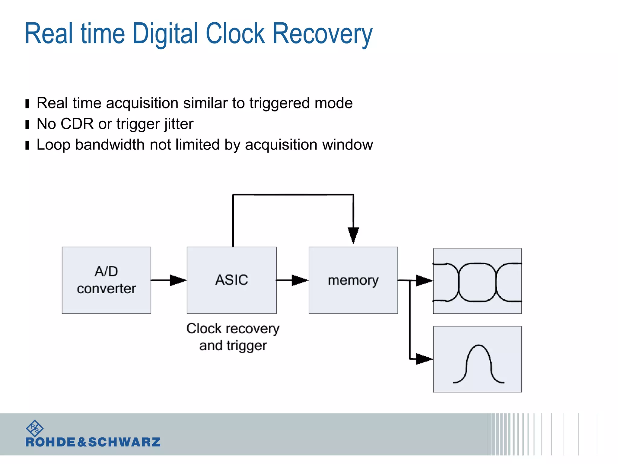
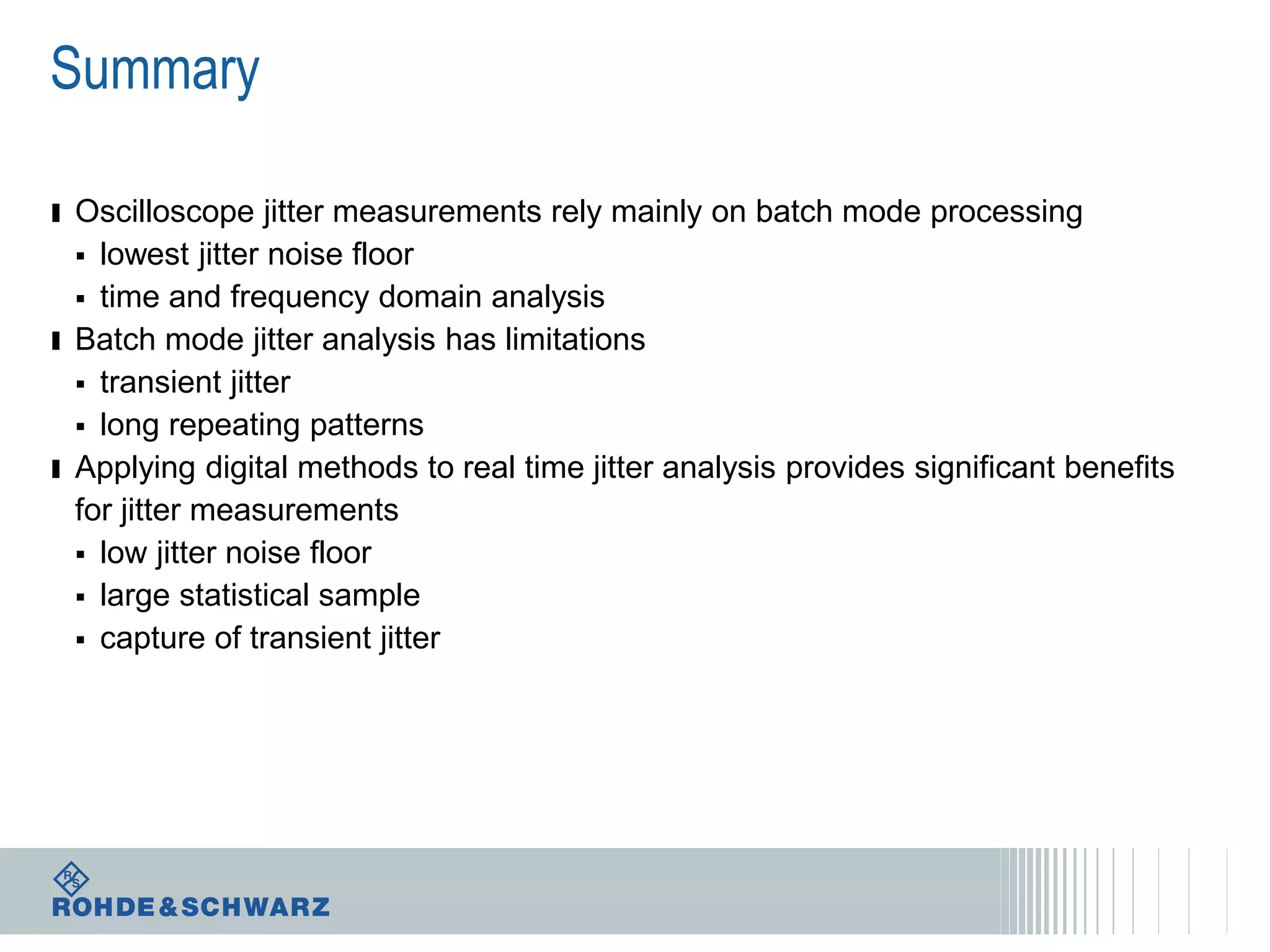
The document details a webinar on jitter measurement methods, highlighting real-time and batch mode measurements, types of jitter, and various measurement instruments. It covers key concepts like time interval error, probability density functions, and dual Dirac jitter models used for analyzing jitter data. The summary emphasizes the importance of oscilloscopes in jitter measurement and the limitations of batch mode processing versus real-time analysis.

1. Real Time Jitter Measurement
Live webinar from 2/11/14
View the On-Demand webinar, http://ubm.io/LywVYU

2. Overview
ı Background jitter measurement methods
Batch mode jitter measurement
 Triggered measurement
 Real –time digital clock recovery
ı Jitter transfer function (real time vs. batch)
ı Transient and low rate jitter events
ı Measurement examples
 Low rate jitter
 PRBS31


3. What is Jitter?
Data
Clk
Setup
Time
Hold
Time
Q
l Jitter includes instability in signal period, frequency, phase, duty cycle or some other timing
characteristic
l Jitter is of interest from pulse to pulse, over many consecutive pulses, or as a longer term
variation
l Very long term variations (<10Hz) are a separate class of pathologies referred to as wander
(Telecommunication only)

4. Serial digital data transmitter

5. Time Interval Error (TIE)
TIE is the difference between the measured clock edge and the ideal clock edge
locations
TIE is essentially the instantaneous phase of the signal

6. Jitter Measurement Instruments
Real time (Oscilloscope)
Single-shot or repetitive events (clock or data)
Bandwidths typically 60 MHz – 30+ GHz
Lowest sensitivity (highest jitter noise floor)
Measures adjacent cycles
Repetitive (Sampling Oscilloscope)
Repetitive events only (clock or data)
Bandwidths typically 20 GHz - 100 GHz
Generally can not discriminate based on jitter frequency
Cannot measure adjacent cycles
Phase noise (Phase noise test set)
Sensitivity
Clock signals only
Must integrate phase noise over frequency to measure jitter
Highest sensitivity (lowest jitter noise floor)
Cannot measure adjacent cycles
Flexibility

7. Spectrum Analyzer Method
7

8. Phase Detector Method
PLL-Controlled Reference
⊗√=90°
DUT
PD
Low Pass
Filter
LNA
Spectrum
Analyzer
PLL
PLL Low Pass Filter
Reference
Source
8

9. Phase Detector Method
Input signals of the mixer (having 90° offset, i.e. in “Quadrature“):
Output signals of the mixer:
After low-pass filtering and assuming ƒL= ƒR we get:
For small changes in phase (simplification allowed for this kind of noise):
9

10. Relationship between phase noise and jitter

11. Timing Measurement in Oscilloscopes
Threshold crossing time
interpolation
threshold
50 ps
50 ps
ı Time is measured at the point where the waveform amplitude crosses a
predefined threshold
ı Samples are spaced at the sample interval (50 ps at 20 Gs/s for example)
ı Sin(x)/x or cubic interpolation is used on the waveform transition followed by
linear interpolation of the points nearest the crossing to find the exact time

12. Jitter Measurement: Histogram
ı Collection of measurements
arranged in an x-y plot value
vs. frequency of occurrence
ı Approximation of a PDF
when normalized
ı Analyzed to "measure" total
jitter and jitter components
(random, deterministic, etc.)

13. Jitter Measurement: Jitter Track
t1
t2
t3
t4
t
t
ı Jitter measurement over time
ı Synchronous sampling with signal transitions
ı Used to measure jitter spectrum
t5

14. Jitter as a Random Variable
ı Jitter is a combination of random and deterministic sources and can be treated
as a random variable
ı The jitter histogram is used as an estimate of the probability density function
(PDF) of the timing values – usually TIE
ı A model is fit to the estimated PDF and is used to predict the range of timing
values for any sample size
 Referred to as the total jitter
 The sample size is defined in terms of an equivalent bit error rate

15. The Random Component of Jitter
# Measurements
100
1,000
5,000
10,000
100,000
1,000,000
5,000,000
100,000,000
1,000,000,000,000
Peak-to
peak (σ)
±2.1
±2.9
±3.4
±3.5
±4.1
±4.6
±5.1
±6.0
±7.0
Theoretically, the peak to peak value of random jitter will grow without bound.
To define the random jitter you must specify a measurement time.

16. Probability Density Functions
ı The PDF is a function that gives the probability that a random variable takes on
a specific value
ı In the case of jitter, this is the probability that a transition happens at a specific
time from its expected location
ı The cumulative density function is the integral of the PDF and gives the total
probability of a transition happening within a certain time range of the expected
transition time
ı The histogram of a random measurement is an estimate of the PDF for that
measurement

17. The Dual Dirac Jitter Model
ı Fit Gaussian curve to the left and
ı
ı
ı
ı
ı
right sides of estimated jitter PDF
(i.e. the measured normalized
histogram)
Separation of the mean values
gives Dj(δ−δ)
Standard deviation gives Rj
Dj(δ−δ) and σ are chosen to best fit
the measured histogram in the tails
Model Predicts jitter for low bit error
rates
Note that the model does not fit the
central part of the measured
distribution

18. Jitter and Bit Error Rate
BER
Jitter PDF
0
UI
1

19. Total Jitter Curve
ı The specified BER is
another way of expressing a
confidence interval or
observation time
ı Total jitter is determined by
integrating the probability
density function (PDF)
separately from the left and
right sides to determine the
cumulative probability
density (CDF)
ı The width of this curve at
the specified BER (or
confidence interval) gives
the total jitter
CDF
(total jitter)
PDF
Total jitter and PDF for a Gaussian distribution
with standard deviation = 1

20. Summary of Histogram Analysis
ı Histograms are used to estimate the PDF of random variables such as jitter
ı Jitter consists of both random and “deterministic” components
Random jitter is assumed to have a Gaussian PDF
 Deterministic jitter is actually bounded and is modeled by a pair of Dirac delta
functions
ı The Dual Dirac model is used to extrapolate a small set of jitter measurements
in order to predict the peak to peak range of a much larger sample
ı The sample size is expressed in terms of bit error rate
 BER of 1e-12 equals a sample size of approximately 2e12 bits
 Ratio of ‘1’ to ‘0’ values is assumed to be ½
ı Rj and Dj from the Dual Dirac jitter model are specified in all serial data
standards for jitter


21. Jitter measurement methods
ı Oscilloscope is the primary instrument for jitter measurement
Measurement of clock and data signals
 Wide range of measurement types (period, cycle to cycle, TIE, etc)
ı Measurement methods used in oscilloscopes
 Real time (triggered)
 Batch mode


22. Real time jitter measurement
ı Hardware clock recovery
ı Separate trigger circuit
ı Timing uncertainty introduced via CDR, trigger and ADC sampling clock

23. Batch Mode Jitter Measurement
ı Analyze long signal acquisition
ı Software clock recovery applied
to timing data
ı Many analysis features
(frequency, time, statistical)

24. Jitter Noise Floor
Batch mode
Typ. 330 fs
Noise
Sampling clock jitter
Triggered
Typ. 1.5 ps
Noise
Sampling clock jitter
Clock recovery jitter
Trigger jitter

25. Real time Digital Clock Recovery
ı Real time acquisition similar to triggered mode
ı No CDR or trigger jitter
ı Loop bandwidth not limited by acquisition window

26. Limitations of Batch Mode Jitter Measurement
ı
ı
ı
ı
Inherent low frequency cutoff due to windowing
Large time gaps in acquisition obscure transient jitter
Generally impossible to measure long stress data patterns
Discontinuous phase tracking can cause phase "slipping"

27. Jitter transfer function
N measurements

28. FFT Bin Response
Jitter transfer function
Each bin has a sin(x)/x response
Low frequency cutoff at the first FFT bin

29. Jitter transfer function
1 MHz carrier with 10 KHz sinusoidal jitter measured over a 100 us time window

30. Jitter transfer function
1 MHz carrier with 10 KHz sinusoidal jitter measured over a 50 us time window

31. Transient jitter

32. Example of transient jitter
histograms of low rate jitter measured using batch and continuous modes. Jitter
Injected at 1/3208 rate

33. Example of Jitter on a Long Pattern
Histograms of jitter measured on a PRBS31 data pattern. The linear trend lines
on the histogram on a log scale estimate the total jitter

34. Summary
ı Oscilloscope jitter measurements rely mainly on batch mode processing
lowest jitter noise floor
 time and frequency domain analysis
ı Batch mode jitter analysis has limitations
 transient jitter
 long repeating patterns
ı Applying digital methods to real time jitter analysis provides significant benefits
for jitter measurements
 low jitter noise floor
 large statistical sample
 capture of transient jitter


35. Learn More
ı For more information on the instruments seen in this presentation, please visit

www.rohde-schwarz-scopes.com
ı If you’re interested in a free demo of our products, please visit

http://www.rohde-schwarz-usa.com/FASTDemo.html