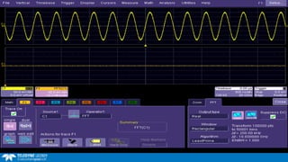
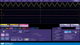
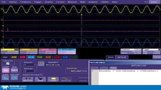
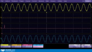
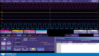
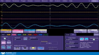
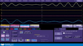
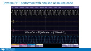
The document discusses how to make custom oscilloscope measurements using MATLAB and VB, detailing various communication configurations and integration methods. It explains the process of creating custom measurements, applying digital filters, and automating analysis through MATLAB's capabilities. Additionally, it includes application examples demonstrating precision measurements and real-time data processing in oscilloscope applications.

1. Making Custom Oscilloscope Measurements
Using MATLAB and VB
April 22nd, 2015

2. Signal Path Block Diagram - from Acquisition to Processing
Amp
Digitized
Waveform
A
D
C
Analog-to-Digital
Converter Display
Processing
Acquisition
Memory
Trigger Circuit
SIMPLIFIED OSCILLOSCOPE BLOCK DIAGRAM
Analog
Waveform

3. Three Possible Communication Configurations
Configuration 1: Remote Control Scope From Computer
Computational results reside in MATLAB software
Scope Platform
GPIB /
ENET
Computer Platform
Scope Software MATLAB

4. Three Possible Communication Configurations
4
Configuration 2: MATLAB Software Installed on Scope
Scope Platform
Scope Software MATLAB
Computational results reside in MATLAB software

5. Three Possible Communication Configurations
Configuration 3: MATLAB Software Integrated Within Scope Application
MATLAB-assisted dynamic collaboration as the
oscilloscope and MATLAB share native capabilities.
Scope Platform
DRIVER
Scope Software
MATLAB
INLINE PROCESSING

6. Three Possible Communication Configurations
Scope Platform
Scope App
Computer Platform
Configuration 1: Remote Control Scope From Computer
GPIB /
ENET
Scope Platform
Scope AppMATLAB
Configuration 2: MATLAB Installed on Scope
Scope Platform
Scope App
Configuration 3: MATLAB Fully Integrated Within Scope Application
Computational results reside in MATLAB software
INLINE PROCESSING
MATLAB-assisted DSO shares native capabilities
Computational results reside in MATLAB software
MATLAB
MATLAB

7. Workflow Model for Incorporating A New Algorithm
Appl
Engr
Prod
Mngr
Contacts applications
Collects data, logs report,
contacts product manager
Engr
Mngr
Dsn
Engr
Evaluates request,
prioritizes projects
Assigns resources,
places project in queue
Already moved on to a different
project, no longer needs
measurement
Six months later, implements
inline measurement into firmware
Releases firmware with
feature included
Notifies local rep
Delivered to end user
End
User
Traditional Model:
Sales
Engr
Requires a new feature;
contacts local
representative with request
Time Scale: 6 - 9 months
Inline Processing Model:
End
User
Incorporates new inline
measurement today, and can
begin to use it immediately
Time Scale: Immediate
Proprietary measurements can remain
classified and do not need to be shared
with scope vendor or the outside world

8. How Is A Measurement Selected?
Traditional parameters
added to the measurement

9. How Is A Custom Measurement Selected?
Allows user-defined in-line
custom measurements
Custom parameters
are added to the
measurement list
just like traditional
parameters

10. Fully-Integrated Custom Measurement
Add your own
customized
measurement or
math function
And the result is
fully integrated into
the scope process
as a measurement
or trace

11. Inline Custom Measurement
Custom MATLAB
parameter finds the time
elapsed for half-life of the
damped sine
The value 3.149 is the
number of cycles that
have occurred when the
signal reaches 50%
of its peak amplitude

12. Real-Time Modification of Custom Measurement
MATLAB dialog box displays MATLAB responses
On-scope editor allows loading, saving, and real-
time modification of script algorithms

13. Arbitrary Waveform Generated on Scope
OutResult.Samples = InResult.Samples
startData = 0
endData = OutResult.Samples
newNumPoints = endData - startData
ReDim newDataArray(OutResult.Samples)
unscaledData = InResult.DataArray(False)
Randomize Timer
Pi = 3.14159 : TwoPi = 2.0 * Pi
WaveLength = 0.02 ' as a fraction of the timebase
WL = WaveLength * newNumPoints
WN = TwoPi / WL
TimeConstant = 0.1 ' as a fraction of the timebase
TC = TimeConstant * newNumPoints
A = 30000
Noise = 100.0
For i = WL To endData - 1
Y = A * (exp(-i/TC)) * sin(WN * i)
Y = Y + Noise * (rnd+rnd+rnd+rnd+rnd+rnd-3.0)
newDataArray(i) = Y
Next
OutResult.DataArray(False) = newDataArray
The damped sinusoid was
simulated mathematically
(scope simulates but does not output waveform)
Waveform now exists in
scope memory buffer

14. Peak Decay Ratio
Custom parameter finds the peak
decay ratio of the damped sinusoid.
The 0.82 reading indicates each peak
in the waveform is 0.82 the amplitude
of the adjacent previous peak.

15. Application Example:
MATLAB Digital Filtering

16. MATLAB Butterworth Filter
Swept Sine
Low Pass Butterworth

17. MATLAB Butterworth Filter
MATLAB Signal
Processing Toolbox
supports up to 500th
order Butterworth filter
This MATLAB filter
was implemented with
only 5 lines of code

18. Wavelet Transforms
WformOut = WformIn1(1:2:end)-WformIn1(2:2:end);
Because of vectorization in MATLAB, a
Haar Wavelet can be performed using
only one line of code:
Applications for Wavelets include filtering, data
compression, and signal processing

19. Notch Filter
Swept Sine
Notch Filtered Swept Sine

20. Example Mixing Mathematical Waveforms with Input
(Real signal captured by the scope with noise added algorithmically)
Pure Mathematical Gaussian Noise
Input Signal
Input Signal + Noise

21. Automatic Leveling Filter
Filter removes slow mean variations by repositioning
waveform data

22. User-designed FFT Windowing
Input signal
Custom window applied to data
FFT is now performed on custom window
Any FFT windowing algorithm can be used with FFT

23. Application Example:
MATLAB Inverse FFT

32. Inverse FFT performed with one line of source code
WformOut = ifft(WformIn1 + j*WformIn2);

33. Application Example:
Graphic Programming with MATLAB

34. Processing Web
Building parameters or math functions from basic building blocks

35. Processing Web
Building parameters or math functions with MATLAB operators

36. Simulink Blocksets Can Be Used for Realtime Simulation

37. Application Example:
Display Techniques

38. 3-D Display of Data
Surface mesh shows progression
of square wave over time

39. Rotating the Surface Viewing Angle
Image vantage point can rotate on 3 axes while viewing this Swept Sine

40. Custom Display Techniques
Waterfalls and 3-D Data Rotation

41. Custom Graphical User Interfaces
Crest Factor is computed and
displayed via a custom MATLAB
graphical user interface

42. Application Examples:
Custom Timing Measurements

43. IEEE Risetime Definition

44. EMC Risetime Custom Definition
EMC Risetime Custom Definition
IEEE Risetime Definition

45. EMC Risetime Custom Definition
Custom EMC Pulse Measurement

46. Crossing Point Between Two Waveforms
 The editor is provided in the scope
application
 In case of error, the status will be set to
error and gives the number of the
concerning line.
 Possible to write the code in a separate
editor and import it
 Export the code to a file
 When saving the setup, the code will be
saved internally for further processing, so
no need to re-write it.
 Crossing point time between two waveforms
 Takes two internal parameters as input and gives one as an output
 The user provides the crossing level in the scope’s time@lvl parameter
 This combination uses the scope’s internal parameters as input

47. Application Example:
Waveform Correlation

49. Waveform Correlation
Customization allows the scope to apply the spreadsheet's
correlation capability for waveform analysis

50. Waveform and measurement results can be "pushed" directly into a spreadsheet
Measurements
on spreadsheet-
generated trace
Trace generated
from spreadsheet
Acquired
Trace

51. Application Example:
Decision Process Math Operators

52. Dynamic Automation Controls
Input
Waveform
Static Result
Continuously Sampled Output
Dynamic Automation Controls

53. MATLAB Dynamic Feedback During Testing
h=actxserver('LeCroy.XStreamDSO');
vertoffset = get(h.Acquisition.C2.VerOffset,'Value')
if (h.PassFail.Q1.Out.Result.Value) == 0 %% mask test fails
vertoffset = get(h.Acquisition.C2.VerOffset,'Value')
if (vertoffset > 0) %% trace offset is positive
set(h.Acquisition.C2.VerOffset,'Value',(vertoffset + 0.005));
else
set(h.Acquisition.C2.VerOffset,'Value',(vertoffset - 0.005));
end
end
3
2
1 Custom scripts can
use Automation
Controls to act as a
feedback mechanism
to modify scope
settings based on
measurement results
This example uses
Automation Controls
to automatically
modify scope
settings and move
waveform clear of
mask region
= automation controls
Mask test
pass/fail result
queried and
scope channel
vertical offset
modified using
Automation

54. Measurement on Trace 1 is Gated by Pulses of Trace 2
This example shows how a measurement definition can be dynamically determined by
the properties of the waveform data itself. In this example, the portion of data where the
measurement takes place on Trace 1 is dependent on the area marked between the two
pulses of Trace 2.

55. Script has not begun computing average because
Pass/Fail condition has not yet been True

56. Script begins averaging F8

57. Averaging continues on acquisitions
only when Pass/Fail condition is True

58. Averaging pauses whenever
Pass/Fail condition is False

59. Averaged waveform takes shape of C1 after
287 sweeps. 79 averages have taken place
because Pass/Fail condition was True 79 out
of 287 sweeps

60. Application Example:
Linear Regression / Slope Intercept

61. Oxygen Depletion in a Muscle Fiber

62. Experiment to measure oxygen depletion in muscle fiber

63. Nitrogen is injected into container to displace oxygen

64. Trend line records oxygen level as a function of time

65. Long-term trend line can be extracted as a waveform

66. Long-term trend line of oxygen vs. time

67. Linear Regression to Determine Slope Intercept
of Oxygen Depletion at t=0

68. Application Example:
Precision Burst Timing

69. A ground-fault circuit interruptor (GCFI) is a device that disconnects a circuit
whenever it detects that the electric current is not balanced between the energized
conductor and the return, and is used to prevent injury caused by electric shocks.
The measurement goal is to determine the exact amount of time that the 60 Hz
cycle is present before the GFCI disables the output, and determine the start, stop,
and duration of the ground fault circuit interrupter tripping time.
Ground fault circuit interruptor
GFCI Test Panel
Ground Fault Circuit Interrupter Tripping Time Measurement

70. The exact start and stop time of each
burst is variable.
The burst length includes non-integer
portions of the waveform cycles.
Ground Fault Circuit Interrupter Tripping Time Measurement Challenge

71. Non-integer portions of the waveform are not
measured by standard measurements (such
as period) by oscilloscopes
Timing measurement example using IEEE pulse parameters

72. GFCI Burst measurement requirement
The use of cursors is not desirable because
the burst length varies for each acquisition and
the replacement of manual cursors by the
operator significantly reduces overall test time
Burst length varies from acquisition to
acquisition and includes non-integer cyclical
values. The exact size and shape of the non-
integer portion is also variable.
Example GFCI burst containing 6+ cyclesExample GFCI burst containing 5+ cycles

73. Zoom at start of burst showing
fine placement of cursor on start
time
Zoom at end of burst showing fine
placement of cursor on stop time
The GFCI burst length varies for each
acquisition. The manual placement of cursors
and zooms (both of which need to be
repositioned for every acquisition by the
operator), is time-consuming and significantly
reduces overall test throughput.

74. Scripting reports accurate burst start and stop time with 1 ns precision
on 100 ms time capture window

75. Scripting dynamic repositions labels and dynamically zooms on every acquisition

76. Measurements-on-statistics shows range, median, mode, etc. of cumulative burst times

77. Script only 416 lines of code, covers all corner case scenarios, calculates burst times,
and dynamically repositions zooms and labels

78. Application Example:
RF Signal Processing

79. Hilbert Transform on 10 GHz RF Burst using In-line MATLAB

80. Hilbert Transform on 10 GHz RF Burst using In-line MATLAB

81. Hilbert Transform on Burst using In-line MATLAB

82. Getting Started Resources

83. Sample MATLAB Routines can be downloaded from LeCroy’s Website
Pre-written math and measurement samples on
Teledyne LeCroy’s web site
www.teledynelecroy.com/MATLAB

84. Application Note: Implementing MATLAB Filters on Waveform Data

85. Application Note: Decoding NRZ Data with MATLAB

86. Application Note: Interfacing with Simulink

87. Application Note: MATLAB COM object programming examples

88. Making Custom Oscilloscope Measurements
Questions?