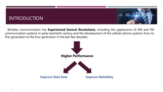
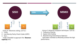
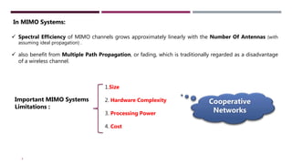
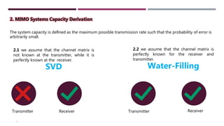
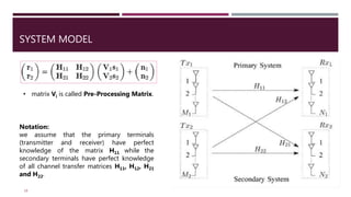
1) The document introduces MIMO (multiple-input multiple-output) wireless communication systems and discusses their advantages over traditional SISO systems, including higher spectral efficiency and ability to benefit from multipath propagation. 2) It describes the MIMO channel model and derives the capacity of MIMO systems using singular value decomposition and water-filling principles. MIMO capacity is shown to increase approximately linearly with the number of antennas. 3) Cooperative communication techniques that enable single-antenna devices to achieve MIMO-like benefits are introduced, along with the concepts of cognitive radio networks and spectrum pooling.

1. IN THE NAME OF GOD
Introduction to MIMO
By:
Mohammad Reza Jabbari
October 20161

2. INTRODUCTION
2
Wireless communication has Experienced Several Revolutions, including the appearance of AM and FM
communication systems in early twentieth century and the development of the cellular phone systems from its
first generation to the four generation in the last few decades.
Higher Performance
Improve Data Rate Improve Reliability

3. 3
SISO MIMO1990s NOW
Using of Advances coding, such as :
1. Turbo
2. Low Density Parity Check Codes (LDPC)
3. And …
made it feasible to approach the Shannon
capacity limit.
Using of Advances reception techniques such as :
1. Frequency Sharing
2. Space-time Coding
3. Beamforming And Antenna Selection
have been invented to efficiently achieve the high
performance.

4. 4
In MIMO Systems:
 Spectral Efficiency of MIMO channels grows approximately linearly with the Number Of Antennas (with
assuming ideal propagation) .
 also benefit from Multiple Path Propagation, or fading, which is traditionally regarded as a disadvantage
of a wireless channel.
Important MIMO Systems
Limitations :
1.Size
2. Hardware Complexity
3. Processing Power
4. Cost
Cooperative
Networks

5. MIMO SYSTEMS
5
1. MIMO Systems Model
 Let us consider a single point-to-point MIMO system with arrays of nT transmit and nR receive antennas.
 The transmitted signals in each symbol
period are represented by an nT×1
column matrix X, where i th component xi
refers to the transmitted signal from
antenna i.

6. 6
 The channel is described by an nR × nT complex matrix, denoted by H. the i j-th component of the matrix
H, denoted by hij, represents the Channel Fading Coefficient from the j th transmit to the i th receive
antenna.
 By using the Linear Model the received vector can be represented as:
 The Noise at the receiver is described by an nR × 1 column matrix, denoted by n. Its components are
statistically independent complex zero-mean Gaussian variables, with independent and equal variance
real and imaginary parts :

7. 7
MIMO SYSTEM CAPACITY
The system capacity is defined as the maximum possible transmission rate such that the probability of error is
arbitrarily small.
2. MIMO Systems Capacity Derivation
2.1 we assume that the channel matrix is
not known at the transmitter, while it is
perfectly known at the receiver.
SVD
2.2 we assume that the channel matrix is
perfectly known for the receiver and
transmitter.
Water-Filling
Transmitter Transmitter ReceiverReceiver

8. 8
2.1 Singular Value Decomposition SVD
Matrix H can be written as:
the eigenvalue of HHH denoted by 𝜆 are defined as :
Notation: The number of nonzero eigenvalues of matrix HHH is equal to the rank of matrix H, denoted by r.
Thus the equivalent MIMO channel can be consisting of r Uncoupled Parallel Sub-Channels. Each sub-
channel is assigned to a singular value of matrix H, which corresponding to the amplitude channel gain. The
channel power gain is thus equal to the eigenvalue of matrix HHH.

9. 9

10. 10
 Note that in the equivalent MIMO channel capacity modeled by the uncoupled sub-channels are their
capacities add up. We can estimate the overall channel capacity, denoted by C, by using the Shannon
capacity formula:
where W is the bandwidth of each sub-channel and Pri is the received signal power in the i th sub-channel.
 Q is the Wishart Matrix defined as:

11. 11
2.2 Water Filling
 Let us consider a MIMO channel where the channel parameters are known at the transmitter. The allocation
of power to various transmitter antennas can be obtained by a “water-filling” principle. The power allocated
to channel i is given by :

12. COOPERATIVE NETWORKS
12
Recently, a new class of methods called Cooperative Communication has been proposed that enables
single antenna mobiles in a multi-user environment to Share Their Antennas and generate a Virtual Multiple-
Antenna transmitter that allows them to achieve transmit diversity and creates a virtual MIMO system.
Cooperation Protocols:
1.Amplify and forward (AF) : Relays act as Analog Repeaters
2.Decode-and-forward (DF) :Relays act as Digital Regenerative Repeaters
3.Compress-and-forward (CF) : Relays Quantize and Compress (Source Coding)

13. COGNITIVE NETWORK (CN)
13
 Cognitive Network is a data communication
network, which consist of Intelligent Devices.
Intelligence means that they are aware of
everything happening inside the device and in the
network they are connected to.
 Cognitive Network is the collection of elements
that make up the network observes network
conditions and then, using prior knowledge
gained from previous interactions with the
network, plans, decides and acts on this
information.
Learning loop by Col John Boyd

14. 14
Spectrum pooling and Space Pooling
However, in some regions, some of the valuable spectrum are under low-efficiency, This is mainly because
the currently fixed Spectrum Allocation policy of today’s wireless networks.
Cognitive radio (CR) technology is widely considered to be one of the most promising technologies for
highly efficient spectrum, which allows the Spectrum Sharing among primary and secondary users in an
Opportunistic Manner .
In spectrum pooling, the spectrum from
different owners is merged into a common
pool, and allowing secondary radio networks
to access the already licensed frequency
bands.
f1
f2
f4
f3
f6
f5
f7
fn

15. 15
Space Pooling

16. PREFACE
We describe a Non-Cooperative Interference Alignment (IA) technique which allows an opportunistic
multiple input multiple output (MIMO) link (secondary) to harmlessly coexist with another MIMO link (primary)
in the same frequency band.
16
Assuming perfect channel knowledge at the primary receiver and transmitter, capacity is achieved by
transmitting along the Spatial Directions (SD) associated with the singular values of its channel matrix using a
Water-filling Power Allocation (PA) scheme.
Often, power limitations (such as low SNR) lead the primary transmitter to leave some of its SD unused.
So Secondary Systems, opportunistically access certain portions of spectrum left unused by other radio
Primary Systems, at a given time or geographical area.

17. 17
Notation: Secondary users should be such that as soon as the primary user wants to use its bandwidth,
bandwidth back to the original owner.
 These pieces of unused spectrum, known as White-Spaces, appear mainly when either transmissions in
the primary network are sporadic, i.e., there are periods over which no transmission takes place, or there
is no network infrastructure for the primary system in a given area, for instance, when there is no primary
network coverage in a certain region. In the case of dense networks, a white-space might be a rare and
short-lasting event
 Private Massage :
Each transmitter sends independent messages only to its respective receiver and no cooperation
between them is allowed, i.e., there is no message exchange between transmitters.
Only One Destination Node Is Able To Decode It.

18. SYSTEM MODEL
18
• matrix Vi is called Pre-Processing Matrix.
Notation:
we assume that the primary terminals
(transmitter and receiver) have perfect
knowledge of the matrix H11 while the
secondary terminals have perfect knowledge
of all channel transfer matrices H11, H12, H21
and H22.

19. INTERFERENCE ALIGNMENT STRATEGY
19
1. Primary Link Performance
primary link must operate at its highest transmission rate in the absence of interference. with singular value
decomposition (SVD) for 𝑯 𝟏𝟏 :
𝐻11 = 𝑈 𝐻11
𝐴 𝐻11
𝑉𝐻11
𝐻
So we can show the optimal pre-processing and post-processing schemes for the primary link to achieve
capacity are given by :
𝑉1 = 𝑉𝐻11
𝐷1 = 𝑈 𝐻11
𝐻

20. 20
Let 𝑚1 = {1.2. ⋯ . 𝑀1} denote the number of transmit dimensions used by the primary User, we know that:
1 ≤ 𝑚1 ≤ 𝑁 where 𝑁 = mi n( 𝑁1 . 𝑀1
The 𝑚1 used dimensions are called Primary Reserved Dimensions, while the remaining 𝑁1 − 𝑚1
dimensions are named Secondary Transmit Opportunities (TO).
The IA strategy, allows the secondary user to exploit these 𝑁1 − 𝑚1 receive dimensions left unused by
the primary link, while avoiding to interfere with the receive dimensions used by the primary link.
𝑆 = 𝑁1 − 𝑚1
2. Secondary Link Performance

21. THE END
21
“Once you stop learning ,you start dying”
Albert Einstein