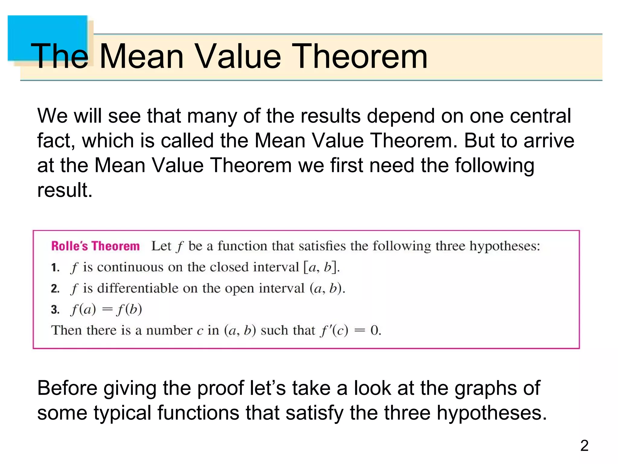
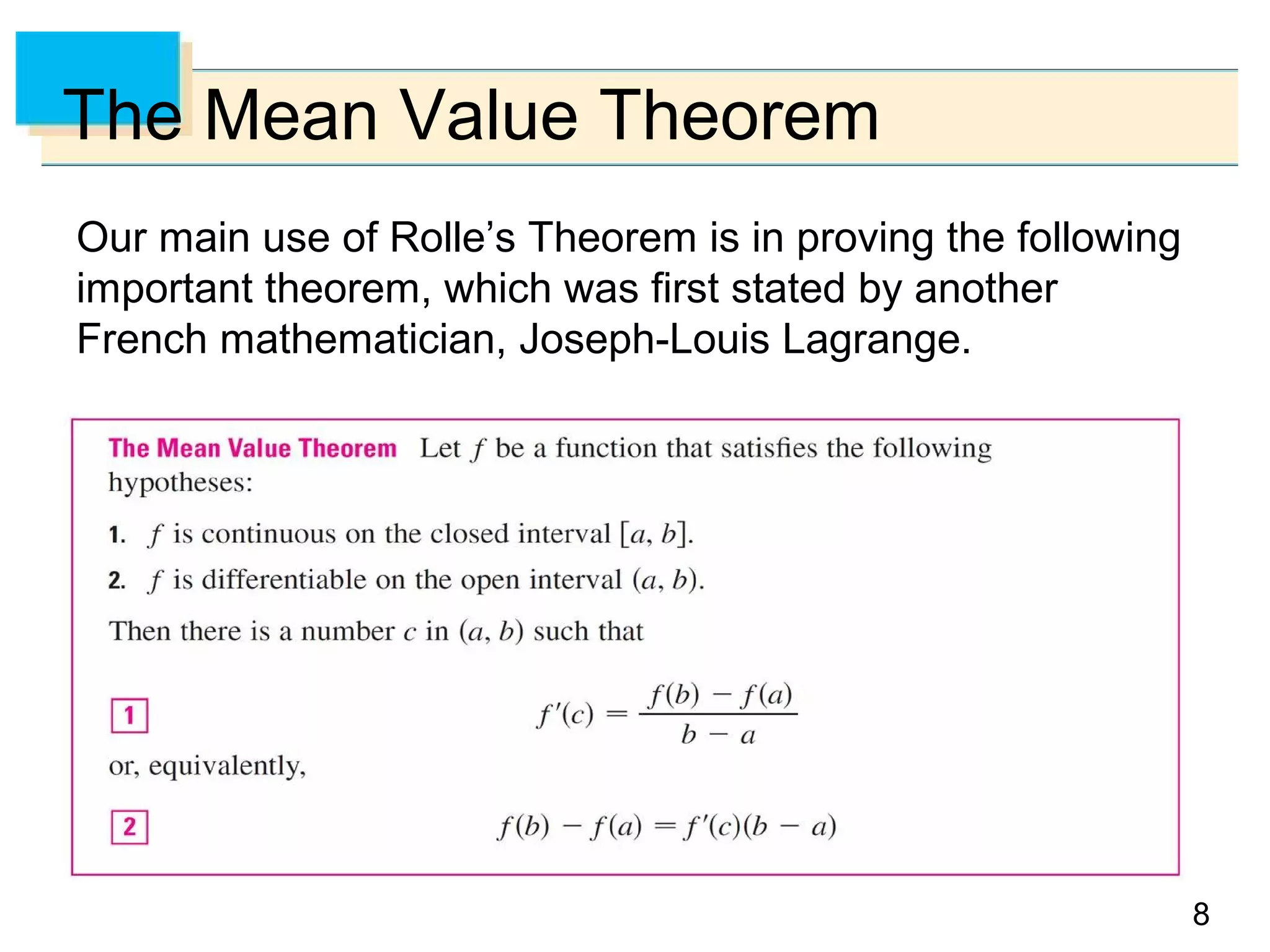
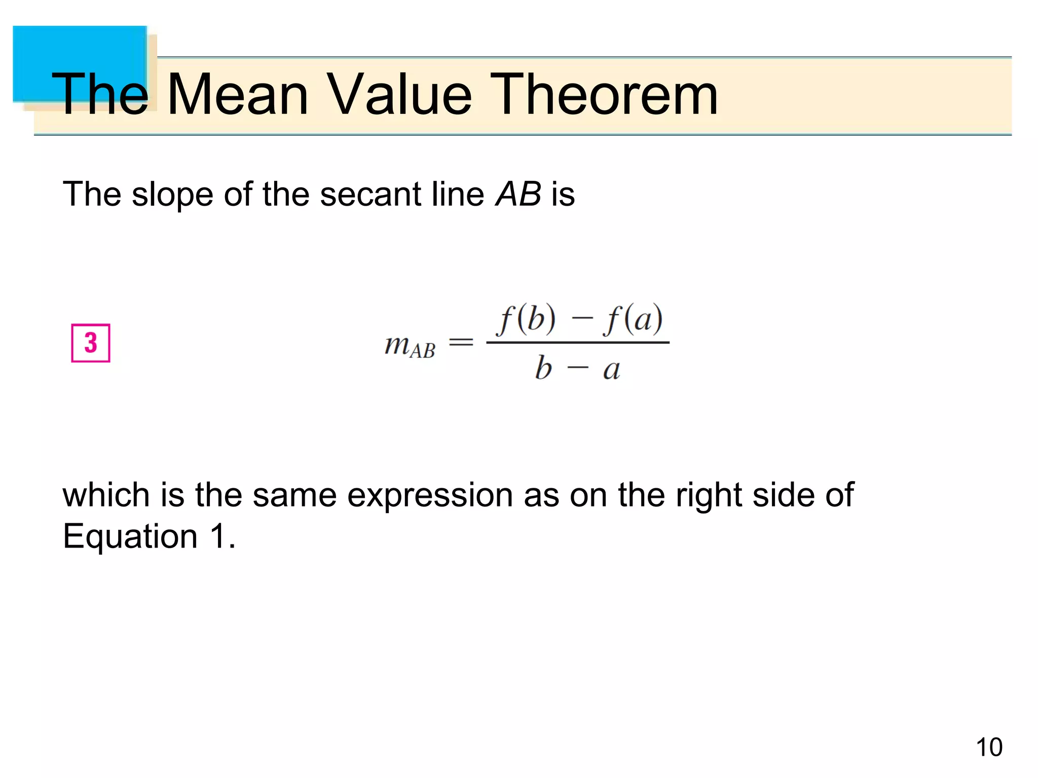
The document discusses the Mean Value Theorem, which states that if a function f(x) is continuous on the closed interval [a,b] and differentiable on the open interval (a,b), then there exists some value c in (a,b) such that: f(b) - f(a) = f'(c)(b - a) In other words, there is at least one point where the slope of the tangent line equals the slope of the secant line between points a and b. The document provides examples and illustrations to demonstrate how to apply the Mean Value Theorem.

1. 4.2
The Mean Value Theorem
Prepared By:
Sheetal Gupta
Asst. Professor
GDRCST, Bhilai

2. 2
The Mean Value Theorem
We will see that many of the results depend on one central
fact, which is called the Mean Value Theorem. But to arrive
at the Mean Value Theorem we first need the following
result.
Before giving the proof let’s take a look at the graphs of
some typical functions that satisfy the three hypotheses.

3. 3
The Mean Value Theorem
Figure 1 shows the graphs of four such functions.
Figure 1
(c)
(b)
(d)
(a)

4. 4
The Mean Value Theorem
In each case it appears that there is at least one point
(c, f(c)) on the graph where the tangent is horizontal and
therefore f′(c) = 0.
Thus Rolle’s Theorem is plausible.

5. 5
Example 2
Prove that the equation x3
+ x – 1 = 0 has exactly one real
root.
Solution:
First we use the Intermediate Value Theorem to show that
a root exists. Let f(x) = x3
+ x – 1. Then f(0) = –1 < 0 and
f(1) = 1 > 0.
Since f is a polynomial, it is continuous, so the Intermediate
Value Theorem states that there is a number c between 0
and 1 such that f(c) = 0.
Thus the given equation has a root.

6. 6
Example 2 – Solution
To show that the equation has no other real root, we use
Rolle’s Theorem and argue by contradiction.
Suppose that it had two roots a and b. Then f(a) = 0 = f(b)
and, since f is a polynomial, it is differentiable on (a, b) and
continuous on [a, b].
Thus, by Rolle’s Theorem, there is a number c between a
and b such that f′(c) = 0.
cont’d

7. 7
Example 2 – Solution
But
f′(x) = 3x2
+ 1 ≥ 1 for all x
(since x2
≥ 0) so f′(x) can never be 0. This gives a
contradiction.
Therefore the equation can’t have two real roots.
cont’d

8. 8
The Mean Value Theorem
Our main use of Rolle’s Theorem is in proving the following
important theorem, which was first stated by another
French mathematician, Joseph-Louis Lagrange.

9. 9
The Mean Value Theorem
Before proving this theorem, we can see that it is
reasonable by interpreting it geometrically. Figures 3 and 4
show the points A(a, f(a)) and B(b, f(b)) on the graphs of
two differentiable functions.
Figure 3 Figure 4

10. 10
The Mean Value Theorem
The slope of the secant line AB is
which is the same expression as on the right side of
Equation 1.

11. 11
The Mean Value Theorem
Since f′(c) is the slope of the tangent line at the point
(c, f(c)), the Mean Value Theorem, in the form given by
Equation 1, says that there is at least one point P(c, f(c)) on
the graph where the slope of the tangent line is the same
as the slope of the secant line AB.
In other words, there is a point P where the tangent line is
parallel to the secant line AB.

12. 12
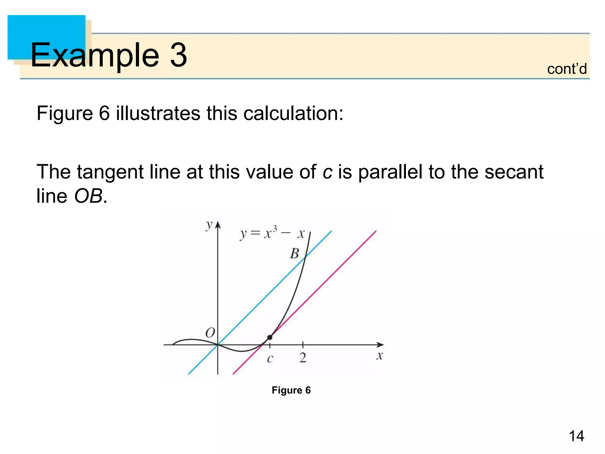
Example 3
To illustrate the Mean Value Theorem with a specific
function, let’s consider
f(x) = x3
– x, a = 0, b = 2.
Since f is a polynomial, it is continuous and differentiable
for all x, so it is certainly continuous on [0, 2] and
differentiable on (0, 2).
Therefore, by the Mean Value Theorem, there is a number
c in (0, 2) such that
f(2) – f(0) = f′(c)(2 – 0)

13. 13
Example 3
Now f(2) = 6,
f(0) = 0, and
f′(x) = 3x2
– 1, so this equation becomes
6 = (3c2
– 1)2
= 6c2
– 2
which gives that is, c = But c must lie in
(0, 2), so
cont’d

14. 14
Example 3
Figure 6 illustrates this calculation:
The tangent line at this value of c is parallel to the secant
line OB.
Figure 6
cont’d

15. 15
Example 5
Suppose that f(0) = –3 and f′(x) ≤ 5 for all values of x.
How large can f(2) possibly be?
Solution:
We are given that f is differentiable (and therefore
continuous) everywhere.
In particular, we can apply the Mean Value Theorem on the
interval [0, 2]. There exists a number c such that
f(2) – f(0) = f′(c)(2 – 0)

16. 16
Example 5 – Solution
so f(2) = f(0) + 2f′(c) = –3 + 2f′(c)
We are given that f′(x) ≤ 5 for all x, so in particular we
know that f′(c) ≤ 5.
Multiplying both sides of this inequality by 2, we have
2f′(c) ≤ 10, so
f(2) = –3 + 2f′(c) ≤ –3 + 10 = 7
The largest possible value for f(2) is 7.
cont’d

17. 17
The Mean Value Theorem
The Mean Value Theorem can be used to establish some
of the basic facts of differential calculus.
One of these basic facts is the following theorem.

18. 18
The Mean Value Theorem
Note:
Care must be taken in applying Theorem 5. Let
The domain of f is D = {x | x ≠ 0} and f′(x) = 0 for all x in D.
But f is obviously not a constant function.
This does not contradict Theorem 5 because D is not an
interval. Notice that f is constant on the interval (0, ) and
also on the interval ( , 0).