Lesson 19: The Mean Value Theorem (Section 021 handout)

Section 4.2
The Mean Value Theorem
V63.0121.021, Calculus I
New York University
November 11, 2010
Announcements
Quiz 4 next week (November 16, 18, 19) on Sections 3.3, 3.4, 3.5, 3.7
Announcements
Quiz 4 next week
(November 16, 18, 19) on
Sections 3.3, 3.4, 3.5, 3.7
V63.0121.021, Calculus I (NYU) Section 4.2 The Mean Value Theorem November 11, 2010 2 / 29
Objectives
Understand and be able to
explain the statement of
Rolle’s Theorem.
Understand and be able to
explain the statement of the
Mean Value Theorem.
Notes
Notes
Notes
1
Section 4.2 : The Mean Value TheoremV63.0121.021, Calculus I November 11, 2010

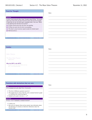
Outline
Rolle’s Theorem
Applications
Why the MVT is the MITC
Functions with derivatives that are zero
MVT and diﬀerentiability
Heuristic Motivation for Rolle’s Theorem
If you bike up a hill, then back down, at some point your elevation was
stationary.
Image credit: SpringSun
Mathematical Statement of Rolle’s Theorem
Theorem (Rolle’s Theorem)
Let f be continuous on [a, b]
and diﬀerentiable on (a, b).
Suppose f (a) = f (b). Then
there exists a point c in (a, b)
such that f (c) = 0.
a b
c
Notes
Notes
Notes
2

Flowchart proof of Rolle’s Theorem
Let c be
the max pt
Let d be
the min pt
endpoints
are max
and min
is c an
endpoint?
is d an
endpoint?
f is
constant
on [a, b]
f (c) = 0 f (d) = 0
f (x) ≡ 0
on (a, b)
no no
yes yes
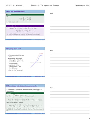
Outline
Rolle’s Theorem
Applications
Heuristic Motivation for The Mean Value Theorem
If you drive between points A and B, at some time your speedometer
reading was the same as your average speed over the drive.
Image credit: ClintJCL
Notes
Notes
Notes
3

Theorem (The Mean Value Theorem)
Let f be continuous on [a, b]
and diﬀerentiable on (a, b).
Then there exists a point c in
(a, b) such that
f (b) − f (a)
b − a
= f (c).
a
b
c
Rolle vs. MVT
f (c) = 0
f (b) − f (a)
b − a
= f (c)
a b
c
a
b
c
If the x-axis is skewed the pictures look the same.
Proof of the Mean Value Theorem
Proof.
The line connecting (a, f (a)) and (b, f (b)) has equation
y − f (a) =
f (b) − f (a)
b − a
(x − a)
Apply Rolle’s Theorem to the function
g(x) = f (x) − f (a) −
f (b) − f (a)
b − a
(x − a).
Then g is continuous on [a, b] and diﬀerentiable on (a, b) since f is. Also
g(a) = 0 and g(b) = 0 (check both) So by Rolle’s Theorem there exists a
point c in (a, b) such that
0 = g (c) = f (c) −
f (b) − f (a)
b − a
.
Notes
Notes
Notes
4

Using the MVT to count solutions
Example
Show that there is a unique solution to the equation x3
− x = 100 in the
interval [4, 5].
Solution
By the Intermediate Value Theorem, the function f (x) = x3
− x must
take the value 100 at some point on c in (4, 5).
If there were two points c1 and c2 with f (c1) = f (c2) = 100, then
somewhere between them would be a point c3 between them with
f (c3) = 0.
However, f (x) = 3x2
− 1, which is positive all along (4, 5). So this is
impossible.
Using the MVT to estimate
Example
We know that |sin x| ≤ 1 for all x. Show that |sin x| ≤ |x|.
Solution
Apply the MVT to the function f (t) = sin t on [0, x]. We get
sin x − sin 0
x − 0
= cos(c)
for some c in (0, x). Since |cos(c)| ≤ 1, we get
sin x
x
≤ 1 =⇒ |sin x| ≤ |x|
Using the MVT to estimate II
Example
Let f be a diﬀerentiable function with f (1) = 3 and f (x) < 2 for all x in
[0, 5]. Could f (4) ≥ 9?
Solution
Notes
Notes
Notes
5

Food for Thought
Question
A driver travels along the New Jersey Turnpike using E-ZPass. The system
takes note of the time and place the driver enters and exits the Turnpike.
A week after his trip, the driver gets a speeding ticket in the mail. Which
of the following best describes the situation?
(a) E-ZPass cannot prove that the driver was speeding
(b) E-ZPass can prove that the driver was speeding
(c) The driver’s actual maximum speed exceeds his ticketed speed
(d) Both (b) and (c).
Outline
Rolle’s Theorem
Applications
Fact
If f is constant on (a, b), then f (x) = 0 on (a, b).
The limit of diﬀerence quotients must be 0
The tangent line to a line is that line, and a constant function’s graph
is a horizontal line, which has slope 0.
Implied by the power rule since c = cx0
Question
If f (x) = 0 is f necessarily a constant function?
It seems true
But so far no theorem (that we have proven) uses information about
the derivative of a function to determine information about the
function itself
Notes
Notes
Notes
6

Most Important Theorem In Calculus!
Theorem
Let f = 0 on an interval (a, b). Then f is constant on (a, b).
Proof.
Pick any points x and y in (a, b) with x < y. Then f is continuous on
[x, y] and differentiable on (x, y). By MVT there exists a point z in (x, y)
such that
f (y) − f (x)
y − x
= f (z) = 0.
So f (y) = f (x). Since this is true for all x and y in (a, b), then f is
constant.
Functions with the same derivative
Theorem
Suppose f and g are two differentiable functions on (a, b) with f = g .
Proof.
Example
Let
f (x) =
−x if x ≤ 0
x2
if x ≥ 0
Is f differentiable at 0?
Solution (from the definition)
We have
lim
x→0−
f (x) − f (0)
x − 0
= lim
x→0−
−x
x
= −1
lim
x→0+
f (x) − f (0)
x − 0
= lim
x→0+
x2
x
= lim
x→0+
x = 0
Since these limits disagree, f is not differentiable at 0.
Notes
Notes
Notes
7

Example
Let
f (x) =
−x if x ≤ 0
x2
if x ≥ 0
Is f differentiable at 0?
Solution (Sort of)
If x < 0, then f (x) = −1. If x > 0, then f (x) = 2x. Since
lim
x→0+
f (x) = 0 and lim
x→0−
f (x) = −1,
the limit lim
x→0
f (x) does not exist and so f is not differentiable at 0.
Why only “sort of”?
This solution is valid but less
direct.
We seem to be using the
following fact: If lim
x→a
f (x)
does not exist, then f is not
differentiable at a.
equivalently: If f is
differentiable at a, then
lim
x→a
f (x) exists.
But this “fact” is not true!
x
y f (x)
f (x)
Differentiable with discontinuous derivative
It is possible for a function f to be differentiable at a even if lim
x→a
f (x)
does not exist.
Example
Let f (x) =
x2
sin(1/x) if x = 0
0 if x = 0
. Then when x = 0,
f (x) = 2x sin(1/x) + x2
cos(1/x)(−1/x2
) = 2x sin(1/x) − cos(1/x),
which has no limit at 0. However,
f (0) = lim
x→0
f (x) − f (0)
x − 0
= lim
x→0
x2 sin(1/x)
x
= lim
x→0
x sin(1/x) = 0
So f (0) = 0. Hence f is differentiable for all x, but f is not continuous at
0!
Notes
Notes
Notes
8

Differentiability FAIL
x
f (x)
This function is differentiable at
0.
x
f (x)
But the derivative is not
continuous at 0!
MVT to the rescue
Lemma
Suppose f is continuous on [a, b] and lim
x→a+
f (x) = m. Then
lim
x→a+
f (x) − f (a)
x − a
= m.
Proof.
Choose x near a and greater than a. Then
f (x) − f (a)
x − a
= f (cx )
for some cx where a < cx < x. As x → a, cx → a as well, so:
lim
x→a+
f (x) − f (a)
x − a
= lim
x→a+
f (cx ) = lim
x→a+
f (x) = m.
Theorem
Suppose
lim
x→a−
f (x) = m1 and lim
x→a+
f (x) = m2
If m1 = m2, then f is differentiable at a. If m1 = m2, then f is not
differentiable at a.
Proof.
We know by the lemma that
lim
x→a−
f (x) − f (a)
x − a
= lim
x→a−
f (x)
lim
x→a+
f (x) − f (a)
x − a
= lim
x→a+
f (x)
The two-sided limit exists if (and only if) the two right-hand sides
agree.
Notes
Notes
Notes
9

Summary
Rolle’s Theorem: under suitable conditions, functions must have
critical points.
Mean Value Theorem: under suitable conditions, functions must have
an instantaneous rate of change equal to the average rate of change.
A function whose derivative is identically zero on an interval must be
constant on that interval.
Notes
Notes
Notes
10

Lesson 19: The Mean Value Theorem (Section 021 handout)

More Related Content

What's hot

Viewers also liked

Similar to Lesson 19: The Mean Value Theorem (Section 021 handout)

More from Matthew Leingang

Recently uploaded

Lesson 19: The Mean Value Theorem (Section 021 handout)