Download as PDF, PPTX

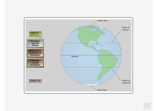


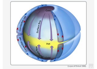
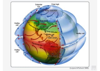
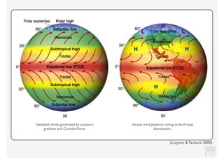
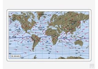
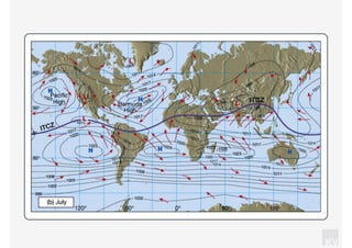
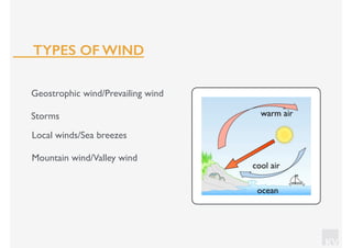
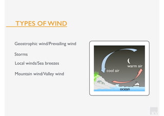
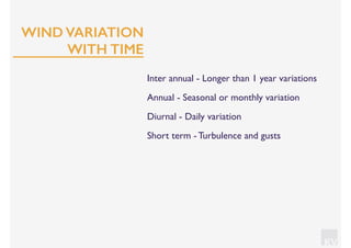
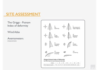
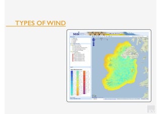
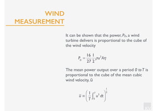


The document provides an overview of wind energy and wind turbine technology. It outlines the objectives to understand wind measurement and analysis, the workings of wind turbines and their components. The key sources and characteristics of wind are described, including types of wind patterns and how wind speed varies with location, time and height. Methods for measuring and analyzing wind resources at potential wind farm sites are also summarized.


