1. The document discusses wind energy quantum and factors that determine the suitability of a location for wind energy generation. These include wind velocity, which must be between 5-25 m/s for optimal turbine operation. Higher wind speeds above 25 m/s can damage turbines. 2. Wind velocity increases with height above the ground according to the power law. Locations near cities or forests have lower wind velocities and are less suitable. The document provides global data on available wind energy, with only 0.06% of land-based wind energy being usable by current technologies. 3. An efficiency factor calculation is shown to determine the actual output of a wind turbine based on the incoming wind power over time. The maximum

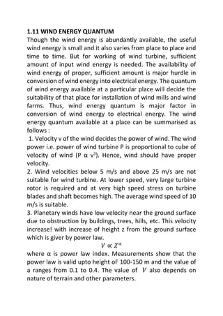
1. 1.11 WIND ENERGY QUANTUM
Though the wind energy is abundantly available, the useful
wind energy is small and it also varies from place to place and
time to time. But for working of wind turbine, sufficient
amount of input wind energy is needed. The availability of
wind energy of proper, sufficient amount is major hurdle in
conversion of wind energy into electrical energy. The quantum
of wind energy available at a particular place will decide the
suitability of that place for installation of wind mills and wind
farms. Thus, wind energy quantum is major factor in
conversion of wind energy to electrical energy. The wind
energy quantum available at a place can be summarised as
follows :
1. Velocity v of the wind decides the power of wind. The wind
power i.e. power of wind turbine P is proportional to cube of
velocity of wind (P α v3
). Hence, wind should have proper
velocity.
2. Wind velocities below 5 m/s and above 25 m/s are not
suitable for wind turbine. At lower speed, very large turbine
rotor is required and at very high speed stress on turbine
blades and shaft becomes high. The average wind speed of 10
m/s is suitable.
3. Planetary winds have low velocity near the ground surface
due to obstruction by buildings, trees, hills, etc. This velocity
increase! with increase of height z from the ground surface
which is giver by power law.
𝑉 ∝ 𝑍∝
where α is power law index. Measurements show that the
power law is valid upto height oF 100-150 m and the value of
a ranges from 0.1 to 0.4. The value of 𝑉 also depends on
nature of terrain and other parameters.

2. 4. Wind velocities are low near cities, forest areas and tall
buildings Therefore, wind farms are located away from them.
5.Some wind energy data to get idea about the quantum of wind
energy available, its usable proportion, all over the world and
India's position in this respect :
6.Total wind energy over the earth is 16.7 x 1012
MWh/year.
7.Wind energy over land area over the earth is 1.67 x 1012
MWh/year i.e. 10% of the total available energy.
8.Usable energy in the world is 0.001 x 1012
MWh/year i.e. only
0.06% of the wind energy available on land area is usable.
9. Table 1.5 gives wind energy data of world and India. This
table shows that wind energy available over land surface is
about 10% of wind energy over the earth. Further, there is
wide scope for installation of wind farms. In India,
measurements of wind speec have been made for many years
at various stations by the India’s Meteorological Department
for assessing overall suitability o-place for locating wind
machines.
Table 1.5
In India, Kandla and Indore are most suitable places for
locating wind machines from the pint of view of energy

3. content in the wind. Generally, locations having annual energy
content greater than 1000 kWh/m2 are considered to be
suitable. There are many such areas along the west and east
coasts as well as Deccan plateau which are suitable for wind
machines.
1.12 WIND POWER DENSITY
Wind power density (Pw) is nothing but the wind energy per
unit time per unit area perpendicular to wind direction at a
given place and at given time and given temperature. It is
directly proportional to the cube of wind velocity or wind
speed (v).
Pw=
E
A−S
where A is area swept in m2
.
and Pw ∝ V3
Pw = KV3
in W/m2
Here, k is conversion factor having S.I. unit Ws3
/m5
. Its
value is k = 0.6386 Ws3
/m5
. Therefore, Pw = 0.6386 v3
.
When the wind energy falls on the blades of the turbine
then it swepts area A. hence the power which is time rate of
winding energy is called incident wind power P and it is written
as
P= Pw.A
The incident wind power drives / rotate the blades and
wind turbine to generate the electrical energy. Further from
above equation the graph of Pw and wind velocity V then its
nature is as shown in Fig. It is called Power-Velocity
characteristics of wind.

4. Fig. 1.3 Power- velocity Characteristics of wind.
1.13 EFFICIENCY FACTOR OF WIND TURBINE (P-H GRAPH)
Energy E in wind of power P in given time interval of h hours
is written as
E = ∫ 𝑃 𝑑ℎ
𝑛
0
(in Wh)
The graph of power of incoming wind (input power Pi) versus
time for a day (24 hours) and that between output power of
wind turbine (output power Po) versus time can be drawn in
the same figure as shown in Fig. 1.4.
From fig. we have following conclusions :-

5. 1)The incident wind power variation (input power) is shown by
curve-I. It increases with time of a day, reaches maximum at
noon (12 hours) and then decreases up to 24 hours. This shows
that power is not obtained at constant rate. The area under
this curve gives energy of wind obtained in 24 hours. It can be
written as (where P = Pi)
Energy of wind in 24 hours = Ew = ∫ 𝑃ℎ. 𝑑ℎ
24
0
= Area under Pi-H curve
(2) Variation of power of turbine (output power Po) versus
time is shown by curve-II. It is seen that this power is less than
incident wind power because the wind machine (turbine)
cannot convert all incident wind energy into useful electrical
energy. A part of wind energy is wasted. The area under curve-
II gives energy output of wind turbine in 24 hours. It can be
expressed as
[𝐸𝑛𝑒𝑟𝑔𝑦 𝑜𝑢𝑡𝑝𝑢𝑡 𝑜𝑓 𝑤𝑖𝑛𝑑 𝑡𝑢𝑟𝑏𝑖𝑛𝑒 𝑖𝑛 24 ℎ𝑜𝑢𝑟𝑠] =
∫ 𝑃𝑜. 𝑑ℎ
24
0
------(1)
=Area under Po-H curve
[Since P = Po]
(3)Point A on curve-II is called cut-in-power point which
corresponds to cut-in-velocity of wind. Below this speed
(power) of wind, the wind machine does not rotate, and no
output power is produced. This is shown by region ABIO under
curve and is wasted power.
(4) Point E on curve-II is cut-out-point which corresponds to
cut-out-speed (power), above which the wind machine cannot
work as the wind with velocity higher than cut-out speed
causes mechanical damage to the machine. Hence it is
required to shut down the machine. Therefore, power

6. obtained at higher velocities of wind is wasted as shown by
area under the curve-II by region EFGH.
(5) Between the points B and E, the velocity (power) of wind
is suitable to produce rated output of wind machine. This
speed of wind between cut-in-speed and cut-out-speed is
called as the design speed of wind. In this case, the output
energy of turbine is given by area under the curve-II shown by
region IBCDEHI. It is written as
[Useful output power of wind turbine in 24 hours] = Area of
region IBCDEHI----(2)
This gives daily energy output of wind turbine.
(6) From equations (2) and (1), the efficiency of wind turbine
is expressed as overall efficiency factor
η =
∫ 𝑃𝑜.𝑑ℎ
24
0
∫ 𝑃ℎ.𝑑ℎ
24
0
% efficiency = η =
∫ 𝑃𝑜.𝑑ℎ
24
0
∫ 𝑃ℎ.𝑑ℎ
24
0
x 100%
(7) The efficiency factor of wind turbine is the ratio of
instantaneous output power Po to instantaneous input power
PI. It is written as Pi
η =
𝑃𝑜
𝑃𝑖
1.14 POWER OF A WIND TURBINE FOR A GIVEN INCOMING
WIND VELOCITY
The most commonly used wind turbine is horizontal axis
propeller type as shown in Fig. 1.5.

7. Fig. 1.5 : Propeller (fan) type horizontal axis wind turbine
blades.
For wind falling normally on the blades of the turbine on inlet
plane 'a' and it leaves the blade on passing through the gaps
between the blades normally from the exit plane (back plane)
'b’.
Let us assume the following :
vi - Velocity of the incoming (incident) wind
ve - Exit velocity of the wind
Pi - Pressure of incoming wind away from plane 'a'
Pa - Pressure of incoming wind at plane 'a'
Pb - Pressure of outgoing wind at plane 'b'
Pe - Pressure of outgoing wind away from plane 'b'
ρ - Density of air
V - Specific volume =
1
ρ
=Volume of unit mass of air
Let there is no loss of energy and no change in density. So we
can write, [Energy per unit mass of incoming wind] =
Pressure energy Pi + K. E. of unit mass of incoming wind
[Energy per unit mass of incoming wind _(i. e. energy at point i)]
= PiV +
1
2
vi
2
− − − − − − − − − − − − − −1)

8. Similar to this equation (1), we can write energy at plane 'a'
as
Energy per unit mass of incoming wind at point a]
= PaV +
1
2
va
2
− − − − − − − − − − − − − −2)
Therefore, from the principle of conservation of energy, we
can write equation for incident side as
PiV +
1
2
vi
2
= PaV +
1
2
va
2
----------------3)
Putting V =
1
ρ
= Specific volume and rearranging, we get
Pi
1
ρ
+
1
2
vi
2
= Pa
1
ρ
+
1
2
va
2
Multiplying by ‘ρ′ we get
Pi +
1
2
ρvi
2
= Pa +
1
2
ρva
2
-----------4)
Similar to equation (4) we can write equation for exit side as
Pb +
1
2
ρvb
2
= Pe +
1
2
ρve
2
-----------5)
From equation (4) and (5), we have
∴ 𝑃𝑎 − 𝑃𝑏= [Pi +
1
2
ρvi
2
−
1
2
ρva
2
] − [Pb +
1
2
ρve
2
−
1
2
ρvb
2
]
∴ 𝑃𝑎 − 𝑃𝑏= [Pi +
1
2
ρ(vi
2
− va
2
)] − [Pb +
1
2
ρ(ve
2
− vb
2
) ]--
---------6)
The pressure and velocity variation of wind at points i, a, b and
e is shown in Fig. 1.6. It shows that wind velocity decreases
from a to b because the kinetic energy of wind is converted
into mechanical work. The incoming velocity v, decreases
gradually as it approaches the turbine and becomes va at inlet
plane 'a'. This wind leaves the blade with velocity vb and at far
distance from plane 'b' at exit point e it becomes ve. Thus vi >
va and vb > ve. Hence from equations (4) and (5), Pa > Pi and Pb

9. < Pe. In other words, the wind pressure rises as it approaches
and decreases as it leaves the blade. Further at long distance
from the blade at points i and e, the pressure is equal i.e. Pe =
Pi
Fig. 1.6 : Pressure and velocity variation at the blade of turbine
Here, thickness of the turbine is very small, velocity within the
turbine does not change va = vb.
Hence equation (6) becomes, [using Pi, = Pe],
∴ 𝑃𝑎 − 𝑃𝑏 = [Pi +
1
2
ρvi
2
−
1
2
ρva
2
− Pe −
1
2
ρve
2
+
1
2
ρva
2
]
∴ 𝑃𝑎 − 𝑃𝑏 =
1
2
ρ(vi
2
− ve
2
)--------7)
The equation (7) gives pressure difference which causes axial
force Fx in the direction of wind. If R is radius or length of blade,
then A = πR2
is the area of propeller on which the pressure
difference acts.
Fx= (𝑃𝑎 − 𝑃𝑏).A=
1
2
ρ(vi
2
− ve
2). A-------------8)

10. But Force = Mass x Acceleration
Fx = mx
dv
dt
=
m
dt
dv
= Air mass flowing per unit time x Change in velocity
However rate of flow of air mass= ρAvt = m
̅-------------------9)
Where vt = vi − ve
∴ m
̅ = ρA(vi − ve)
∴ Fx = ρA(vi − ve) vt-----------------------10)
Comparing equation(8) and (10)
ρA(vi − ve)vt =
1
2
ρ(vi
2
− ve
2). A
vt =
1
2
(vi + ve)----------------------(11)
For thermodynamics system bounded byi and e ,change in
potential energy is zero,change in internal energy is zero,floe
energy (Piv =Pev) is zero. Hence the work done by force in
equation (8) is expressed in terms ofkinetic energy (K.E) as
W= (K.E)i- (K.E)e For unit mass
W=
1
2
(vi
2
− ve
2)------------(12)
Hence, power supplied with mass rate of flow m
̅ is
𝑃 =
𝑊
𝑡
=
1
2
m
̅(vi
2
− ve
2) Use equations (9) and (11),
𝑃 =
1
4
ρA(vi + ve)(vi
2
− ve
2)---------------(13)
In this equation (13), ve is positive in one term and negative in
other term. Hence to find optimum value of velocity ve for a
given vi differentiate equation (13) with respect to ve and
equate it to zero.
i.e
dP
dve
= 0 So we get optimum value of ve = (ve)opt as ve
dP
dve
= 0 =
1
4
ρA{[o + 1][vi
2
– ve
2] + (vi + ve)[0 − 2ve]}
0 = [-3𝑣𝑒2
− 2𝑣𝑖𝑣𝑒 + 𝑣𝑒2
]

11. 3𝑣𝑒2
+ 2𝑣𝑖𝑣𝑒 − 𝑣𝑒2
= 0 -------------(14)
This equation (14) is quadratic in ve.
(𝑣𝑒)𝑜𝑝𝑡 =
−2𝑣𝑖 ± √4𝑣𝑖
2 + (4𝑥3)𝑣𝑖
2
2𝑥3
(𝑣𝑒)𝑜𝑝𝑡 =
−2𝑣𝑖 ± 4𝑣𝑖
2𝑥3
(𝑣𝑒)𝑜𝑝𝑡 =
𝑣𝑖
3
-------- (15)
Thus, maximum power from equation (15) is written as
Pmax =
1
4
ρA(Vi+
vi
3
)(Vi2
−
vi
9
2
)
Pmax =
1
4
ρA
4
3
vi
8
9
vi
2
Pmax =
8
27
ρAvi
3
This equation gives maximum power obtained from wind
turbine for given incoming velocity vi and i.e. is proportional to
the cube of incoming wind velocity vi.