This document provides an introduction to wavelets and their applications. It includes chapters on the mathematical framework of wavelets, fast wavelet algorithms, common wavelet families, and designing wavelets. The chapters cover topics such as continuous and discrete wavelet transforms, orthonormal and biorthogonal wavelet bases, fast wavelet transforms, families like Daubechies and Meyer wavelets, and constructing new wavelets. Examples throughout illustrate wavelet analysis of signals and images.


![Part of this book adapted from “Les ondelettes et leurs applications” published in France by
Hermes Science/Lavoisier in 2003
First published in Great Britain and the United States in 2007 by ISTE Ltd
Apart from any fair dealing for the purposes of research or private study, or criticism or
review, as permitted under the Copyright, Designs and Patents Act 1988, this publication may
only be reproduced, stored or transmitted, in any form or by any means, with the prior
permission in writing of the publishers, or in the case of reprographic reproduction in
accordance with the terms and licenses issued by the CLA. Enquiries concerning reproduction
outside these terms should be sent to the publishers at the undermentioned address:
ISTE Ltd ISTE USA
6 Fitzroy Square 4308 Patrice Road
London W1T 5DX Newport Beach, CA 92663
UK USA
www.iste.co.uk
© ISTE Ltd, 2007
© LAVOISER, 2003
The rights of Michel Misiti, Yves Misiti, Georges Oppenheim and Jean-Michel Poggi to be
identified as the authors of this work have been asserted by them in accordance with the
Copyright, Designs and Patents Act 1988.
Library of Congress Cataloging-in-Publication Data
Wavelets and their applications/edited by Michel Misiti ... [et al.].
p. cm.
"Part of this book adapted from "Les ondelettes et leurs applications"
published in France by Hermes Science/Lavoisier in 2003.
ISBN-13: 978-1-905209-31-6
ISBN-10: 1-905209-31-2
1. Wavelets (Mathematics) I. Misiti, Michel.
QA403.3.W3625 2006
515'.2433--dc22
2006032725
British Library Cataloguing-in-Publication Data
A CIP record for this book is available from the British Library
ISBN: 978-1-905209-31-6
Printed and bound in Great Britain by Antony Rowe Ltd, Chippenham, Wiltshire.](https://image.slidesharecdn.com/03-misiti-waveletsandtheirapplications-220602130041-0d67589d/85/03-Misiti_-_Wavelets_and_Their_Applications-pdf-4-320.jpg)


![Notations xv
LoR Low-pass reconstruction filter
HiR High-pass reconstruction filter
2
↓
or
dec
Down-sampling operator: [ ]
( ) 2
Y dec X X
= = ↓ with 2
n n
Y X
=
2
↑
or
ins
Up-sampling operator: [ ]
( ) 2
Y ins X X
= = ↑
avec 2 n
n
Y X
= and 2 1 0
n
Y + =
∗ Convolution operator: Y X F
= ∗ avec n n k k
k
Y X F
−
∈
= ∑
( )
p
δ
Sequence defined by ( )
0
p
k
δ = if k p
≠ and ( )
1
p
p
δ = for
,
p k ∈
p
T
Translation operator for sequences
( )
p
b T a
= is the sequence defined by k k p
b a −
= for ,
p k ∈](https://image.slidesharecdn.com/03-misiti-waveletsandtheirapplications-220602130041-0d67589d/85/03-Misiti_-_Wavelets_and_Their_Applications-pdf-15-320.jpg)

![Introduction
Wavelets
Wavelets are a recently developed signal processing tool enabling the analysis on
several timescales of the local properties of complex signals that can present non-
stationary zones. They lead to a huge number of applications in various fields, such
as, for example, geophysics, astrophysics, telecommunications, imagery and video
coding. They are the foundation for new techniques of signal analysis and synthesis
and find beautiful applications to general problems such as compression and
denoising.
The propagation of wavelets in the scientific community, academic as well as
industrial, is surprising. First of all, it is linked to their capacity to constitute a tool
adapted to a very broad spectrum of theoretical as well as practical questions. Let us
try to make an analogy: the emergence of wavelets could become as important as
that of Fourier analysis. A second element has to be noted: wavelets have benefited
from an undoubtedly unprecedented trend in the history of applied mathematics.
Indeed, very soon after the grounds of the mathematical theory had been laid in the
middle of the 1980s [MEY 90], the fast algorithm and the connection with signal
processing [MAL 89] appeared at the same time as Daubechies orthogonal wavelets
[DAU 88]. This body of knowledge, diffused through the Internet and relayed by the
dynamism of the research community enabled a fast development in numerous
applied mathematics domains, but also in vast fields of application.
Thus, in less than 20 years, wavelets have essentially been imposed as a fruitful
mathematical theory and a tool for signal and image processing. They now therefore
form part of the curriculum of many pure and applied mathematics courses, in
universities as well as in engineering schools.](https://image.slidesharecdn.com/03-misiti-waveletsandtheirapplications-220602130041-0d67589d/85/03-Misiti_-_Wavelets_and_Their_Applications-pdf-17-320.jpg)


![Introduction xxi
The examples and graphs presented throughout the book have been obtained due
to the MATLAB© Wavelet Toolbox1, which is a software for signal or image
processing by wavelets and packages of wavelets, developed by the authors [MIS
00].
Is our presentation of the development of wavelets timely? Despite our best
efforts, the rate of appearance of applications tests renders any static assessment null
and void. Between 1975 and 1990 mathematical results have appeared in large
numbers, but today they are much fewer. Applications have evolved following a
complementary movement and the quantity of applied work has currently become
very large. Moreover, we can imagine that a considerable number of industrial
applications have not been made public.
Bibliographical references
Let us quote some references offering complete introductions to the domain of
wavelets from the mathematical point of view as well as from the point of view of
signal processing.
Let us start first of all with books strictly dedicated to mathematical processing.
The book by Daubechies [DAU 92] remains from this point of view, a reference
text, along with those of Meyer [MEY 90] and of Kaiser [KAI 94]. These may be
supplemented by two books [FRA 99] and [WAL 02], of greater accessibility and
with a certain teaching potential. Still in the same spirit, but concentrating on more
specific questions, we may consult [COH 92a] on bi-orthogonal wavelets and, for
continuous analysis, we may refer to [TEO 98] and [TOR 95].
The book by Mallat [MAL 98] is, without a doubt, one of the most
comprehensive that is currently available and constitutes an invaluable source, in
particular for those looking for a presentation harmoniously uniting mathematics and
signal.
In the book by Strang and Nguyen [STR 96] an original vision deliberately
directed towards signal processing is adopted. Moreover, it can also be referred to
for concepts and definitions traditional in this field and not presented in this book.
A compact presentation accessible to a large audience can be found in the book
of scientific popularization [MEY 93]. Lastly, in the book by Burke Hubbard [BUR
95] a very enthralling text on the history of the wavelets can be found.
1 MATLAB© is a trade mark of The MathWorks, Inc., 3 Apple Hill Drive, Natick, MA,
01760-2098, USA, info@mathworks.com.](https://image.slidesharecdn.com/03-misiti-waveletsandtheirapplications-220602130041-0d67589d/85/03-Misiti_-_Wavelets_and_Their_Applications-pdf-21-320.jpg)
![xxii Wavelets and their Applications
Naturally, more specialized references deserve to be mentioned: for example,
[COI 92] and [WIC 94] for wavelet packets and [ARN 95], [ABR 97] for interesting
applications of the continuous transform to turbulence or signals presenting
properties of self-similarity.
With respect to denoising and, more widely, the use of wavelets in statistics,
some of the typical results in this field may be found in four very different books
[HAR 98, OGD 97, PER 00, VID 99]. Moreover, we can also refer to [ANT 95] in
order to grasp the extent of the stimulation exerted by the ideas propelled by
wavelets in the statisticians’ community since a few years ago. This latter point can
be usefully supplemented by two more recent articles: [ANT 97] and [ANT 01].
For compression and, in particular compression of images, we may refer to
[DEV 92] for general ideas, to [BRI 95] for application to fingerprints and [USE 01]
and [JPE 00] for the standard JPEG 2000.
Let us mention, finally, that at the end of Chapter 9 a list of books exclusively
devoted to the applications of wavelets can be found.
This book has benefited from lessons on wavelets taught by the authors at the
Ecole centrale de Lyon, at the Ecole nationale supérieure des techniques avancées
(ENSTA), at the mathematical engineering DESS (equivalent to MSc) at the
University of Paris XI, Orsay, at the Fudan University of Shanghai and at the
University of Havana.
The authors would like to express their particular gratitude to Liliane Bel,
Nathalie Chèze, Bernard Kaplan and Bruno Portier for reading this work attentively
and questioningly. Of course, the authors remain responsible for the remaining
errors.](https://image.slidesharecdn.com/03-misiti-waveletsandtheirapplications-220602130041-0d67589d/85/03-Misiti_-_Wavelets_and_Their_Applications-pdf-22-320.jpg)
![Chapter 1
A Guided Tour
1.1. Introduction
In this first chapter1, we propose an overview with a short introduction to
wavelets. We will focus on several applications with priority given to aspects related
to statistics or signal and image processing. Wavelets are thus observed in action
without preliminary knowledge. The chapter is organized as follows: apart from the
introduction to wavelets, each section centers on a figure around which a comment
is articulated.
First of all, the concept of wavelets and their capacity to describe the local
behavior of signals at various time scales is presented. Discretizing time and scales,
we then focus on orthonormal wavelet bases making it possible at the same time:
– to supplement the analysis of irregularities with those of local approximations;
– to organize wavelets by scale, from the finest to the coarsest;
– to define fast algorithms of linear complexity.
Next we treat concrete examples of real one-dimensional signals and then two-
dimensional (images) to illustrate the three following topics:
– analysis or how to use the wavelet transform to scan the data and determine the
pathways for a later stage of processing. Indeed, wavelets provide a framework for
signal decomposition in the form of a sequence of signals known as approximation
1 This chapter is a translated, slightly modified version of the [MIS 98] article published in
the French scientific journal, Journal de la Société Française de Statistique, which the
authors thank for their kind authorization.](https://image.slidesharecdn.com/03-misiti-waveletsandtheirapplications-220602130041-0d67589d/85/03-Misiti_-_Wavelets_and_Their_Applications-pdf-23-320.jpg)

![A Guided Tour 3
reinforced by requiring that the wavelet has m vanishing moments, i.e. verify
( ) 0
k
t t dt
ψ =
∫ for 0, ,
k m
= … .
A sufficient admissibility condition that is much simpler to verify is, for a real
wavelet ψ, provided by:
ψ , 1 2
L L
ψ ∈ ∩ , 1
t L
ψ ∈ and ( ) 0
t dt
ψ =
∫R
To consolidate the ideas let us say that during a certain time a wavelet oscillates
like a wave and is then localized due to a damping. The oscillation of a wavelet is
measured by the number of vanishing moments and its localization is evaluated by
the interval where it takes values significantly different from zero.
From this single function ψ using translation and dilation we build a family of
functions that form the basic atoms:
( ) ( )
,
1
,
a b
t b
t a b
a a
ψ ψ +
−
= ∈ ∈
For a function f of finite energy we define its continuous wavelet transform by
the function f
C :
( ) ( ) ( )
,
,
f a b
C a b f t t dt
ψ
= ∫
Calculating this function f
C amounts to analyzing f with the wavelet ψ . The
function f is then described by its wavelet coefficients ( )
,
f
C a b , where a +
∈ R
and b ∈ R . They measure the fluctuations of function f at scale a . The trend at
scale a containing slower evolutions is essentially eliminated in ( )
,
f
C a b . The
analysis in wavelets makes a local analysis of f possible, as well as the description
of scale effects comparing the ( )
,
f
C a b for various values of a . Indeed, let us
suppose that ψ is zero outside of [ ]
,
M M
− + , so ,
a b
ψ is zero outside the interval
[ ]
,
Ma b Ma b
− + + . Consequently, the value of ( )
,
f
C a b depends on the values of
f in a neighborhood of b with a length proportional to a .
In this respect let us note that the situation with wavelets differs from the Fourier
analysis, since the value of the Fourier transform ˆ( )
f ω of f in a point ω depends
on the values of f on the entire . Qualitatively, large values of ( )
,
f
C a b provide
information on the local irregularity of f around position b and at scale a . In this](https://image.slidesharecdn.com/03-misiti-waveletsandtheirapplications-220602130041-0d67589d/85/03-Misiti_-_Wavelets_and_Their_Applications-pdf-25-320.jpg)
![4 Wavelets and their Applications
sense, wavelet analysis is an analysis of the fluctuations of f at all scales.
Additional information on quantifying the concept of localization and the
comparison between the Fourier and wavelet analyses may be found in [MAL 98] or
in [ABR 97].
The continuous transform (see, for example, [TOR 95] or [TEO 98]) defined
above makes it possible to characterize the Holderian regularity of functions and its
statistical use for the detection of transient phenomena or change-points fruitful (see
Chapter 6).
In many situations (and throughout this chapter) we limit ourselves to the
following values of a and b :
2
= 2 , 2 = for ( , )
j j
a b k ka j k
= ∈|
In this case and for wavelets verifying stronger properties than merely the
admissibility condition – in particular, in the orthogonal case (specified below),
which we shall consider from now on – a function called a scaling function and
denoted ϕ is associated with ψ . We dilate and translate it as ψ . On the whole, the
ϕ function is for local approximations what the ψ function is for fluctuations
around the local approximation, also called the local trend.
We then define the basic atoms of wavelets which are also sometimes called
wavelets:
2
2
,
2
2
,
( ) 2 (2 ), for ( , )
( ) 2 (2 ), for ( , )
j
j
j k
j
j
j k
x x k j k
x x k j k
−
−
−
−
⎧
= − ∈
⎪
⎪
⎨
⎪
= − ∈
⎪
⎩
|
|
ψ ψ
ϕ ϕ
In this context, the wavelet coefficients of a signal s are provided by
( ) ( )
, ,
j k j k
s t t dt
α ψ
= ∫](https://image.slidesharecdn.com/03-misiti-waveletsandtheirapplications-220602130041-0d67589d/85/03-Misiti_-_Wavelets_and_Their_Applications-pdf-26-320.jpg)
![A Guided Tour 5
and, under certain conditions (verified for orthogonal wavelets), these coefficients
are enough to reconstruct the signal by:
( ) ( )
, ,
j k j k
j k
s t t
α ψ
∈ ∈
= ∑ ∑
The existence of a function ψ such that the family { }( ) 2
, ,
j k j k
ψ
∈
is an
orthonormal basis of ( )
2
L is closely related to the concept of multi-resolution
analysis (MRA) (see [MEY 90], [MAL 89] and [MAL 98], and also Chapter 2). An
MRA of the space ( )
2
L of finite energy signals is a sequence { }
j j
V
∈
of nested
closed subspaces:
0
2 1 1 2
V V V V V
− −
⊂ ⊂ ⊂ ⊂ ⊂ ⊂
of ( )
2
L whose intersection is reduced to { }
0 and the union is dense in ( )
2
L .
These spaces are all deduced from the “central” space 0
V by contraction (for 0
j < )
or dilation (for 0
j > ), i.e.:
1
( ) (2 ) for
j j
f t V f t V j
−
∈ ⇔ ∈ ∈|
Lastly, there is a function ϕ of 0
V , which generates 0
V by integer translations,
that is so that:
( ) ( ) ( ) ( )
2 2
0 , ( )
k k
k
V f L f t e t k e l
ϕ
∈
⎧ ⎫
⎪ ⎪
⎪ ⎪
= ∈ = − ∈
⎨ ⎬
⎪ ⎪
⎪ ⎪
⎩ ⎭
∑
where the ϕ function is the scaling function introduced above.](https://image.slidesharecdn.com/03-misiti-waveletsandtheirapplications-220602130041-0d67589d/85/03-Misiti_-_Wavelets_and_Their_Applications-pdf-27-320.jpg)


![8 Wavelets and their Applications
In a column we pass from one filter to another taking the mirror filter, and in a
row we pass from one filter to another taking the mirror filter and multiplying the
even-indexed terms by –1. Thus, just one of these four filters is enough to produce
all the others. Similarly, we can show that on the basis of a given MRA and, thus, of
the scaling function, we can construct the wavelet.
The filters appear in the relations concerning the basic functions associated with
successive levels. These are the equations on two following scales:
1,0 ,
j k j k
k
h
ϕ ϕ
+
∈
= ∑ and 1,0 ,
j k j k
k
g
ψ ϕ
+
∈
= ∑
The sequence h determines the filters of the first column and the sequence g
determines those of the second column.
The wavelet presented in Figure 1.1 forms part of a family of dbn wavelets
indexed by n ∗
∈ introduced by I. Daubechies in 1990 (see Chapter 4 for the
construction). The wavelet db1 is simply the Haar wavelet.
The main properties of the dbn wavelet are as follows:
− it is an orthogonal wavelet, associated with an MRA;
− it has compact support [0, 2n – 1] and the associated filters are of length 2n ;
− the number of vanishing moments is n and, in general, it is far from
symmetric;
− the regularity is 0, 2n when n is sufficiently large.
1.2.3. Organization of wavelets
Wavelets are thus organized using two parameters:
− time k making it possible to translate the forms for a given level;
− scale 2j
making it possible to pass from a level j to the immediately lower
level in the underlying tree represented in Figure 1.2.
In the first column of the figure we find the dyadic dilates (2 times, 4 times, 8
times, etc.) of the scaling function ϕ and in the second column, those of the wavelet
ψ .](https://image.slidesharecdn.com/03-misiti-waveletsandtheirapplications-220602130041-0d67589d/85/03-Misiti_-_Wavelets_and_Their_Applications-pdf-30-320.jpg)


![12 Wavelets and their Applications
This sum defines what will be referred to as the approximation at level J of the
signals . Moreover:
j
J
j J
s A D
≤
= + ∑
This relation means thats is the sum of its approximation J
A and of the finer
details. It can be deduced from it that the approximations are linked by:
1
J J J
A A D
− = +
In the orthogonal case, the family { }
, ,
j k j k
ψ
∈
is orthogonal and we have:
− J
A is orthogonal to 1 2
, , ,
J J J
D D D
− − ;
− s is the sum of two orthogonal signals: J
A and j
j J
D
≤
∑ ;
− the quality J
Q of the approximation of s by J
A is equal to
2
2
J
J
A
Q
s
= and
we have
2
1 2
J
J J
D
Q Q
s
− = + .
1.3. An electrical consumption signal analyzed by wavelets
As a first example we consider a minute per minute record of the electrical
consumption of France; the problem is presented in detail in [MIS 94].
In Figure 1.4 we find, from top to bottom, the original signal (s), the
approximation at level 5 (a5) and the details from the coarsest level (d5) to the finest
level (d1). All the signals are expressed in the same of time unit, which allows a
synchronous reading of all the graphs. The wavelet used is db3.
The analyzed signal represents to the nearest transformation three days of
electrical consumption during summer in France. The three days are Thursday
followed by Friday, having very similar shape and amplitude, then Saturday, which](https://image.slidesharecdn.com/03-misiti-waveletsandtheirapplications-220602130041-0d67589d/85/03-Misiti_-_Wavelets_and_Their_Applications-pdf-34-320.jpg)


![A Guided Tour 17
Let us start by examining the first column and concentrate on the portion of the
signal corresponding to the x-coordinates from 200 to 1,000. Starting from a1 let us
seek, ascending, a level such that the approximation constitutes a good candidate to
be an estimator of the useful signal. Levels 4 and 5 are reasonable. Nevertheless, the
estimator associated with a4 is clearly very bad for the beginning of the signal
corresponding to the x-coordinates 0 to 100. Conversely, an acceptable restitution at
the beginning of the signal would result in choosing a2, which is visibly too noisy.
Let us now look at the details. Detail d1 seems to consist entirely of noise while
details d2 to d5 present large values concentrated at the x-coordinates from 0 to 300.
This is also visible on the graph of the wavelet coefficients (cfs), the largest in
absolute value being the clearest. This form stems from the fact that the signal is a
sinusoidal function with amplitude and period growing with time. The oscillations at
the smallest scales explain the displayed details; the others are in the a5
approximation.
Thus, a plausible denoising strategy consists of:
− keeping an approximation such that the noise is absent or at least very
attenuated (a4 or a5);
− supplementing this approximation by parts of the finer details clearly
ascribable to the useful signal and rejecting the parts which are regarded as
stemming from the noise.
This is precisely what the denoising by wavelets methods achieve, but in an
automatic fashion. The ad hoc choice suggested for this particular simulated signal
is that carried out by one of the most widespread methods of denoising by wavelets
according to Donoho and Johnstone (see [DON 94], [DON 95a], [DON 95b]).
1.6. A Doppler signal denoised by wavelets
Let us consider Figure 1.7. The screen is organized in two columns. In the first
we see wavelet coefficients from level 5 to level 1. To make them more readable,
they are “repeated” 2k
times at level k (which explains the sequences of a constant
gray level especially visible for 3
k > ).
In each one of these graphs we note the presence of two horizontal dotted lines:
the coefficients inside the tube are zeroed by the process of denoising. In the second
column at the top the noisy signal s is superimposed over the denoised signal. In
the middle we find a color version of the wavelet coefficients from level 1 to 5 of
the original noisy signal and in the graph at the bottom the counterpart for the](https://image.slidesharecdn.com/03-misiti-waveletsandtheirapplications-220602130041-0d67589d/85/03-Misiti_-_Wavelets_and_Their_Applications-pdf-39-320.jpg)


![30 Wavelets and their Applications
resolution analysis of the space of the finite energy signals. This provides a
framework for the decomposition of a signal in the form of a succession of
approximations with decreasing resolution, supplemented by a sequence of details.
We then present the bases of wavelet packets, which constitute a generalization
of the orthonormal wavelet bases making it possible, at the same time, to improve
the frequency resolution of the analysis in wavelets and to propose a richer analysis
associated with a large collection of decompositions. It is then possible to select the
decomposition best adapted to a given signal, with respect to an entropy criterion.
Lastly, we introduce the biorthogonal wavelet bases whose idea is to slacken the
strong constraints that an orthonormal wavelet basis must verify. The key is to
consider two wavelets instead of just one. The duality links between the analyzed
and synthesized wavelets are loose enough to partially uncouple the properties of
each of the two bases depending on the objectives.
This chapter outlines a theoretical framework without providing the proofs and
the results are not always expressed in a “tight” mathematical language. Let us then
finish this introduction with some bibliographical indications. The issues discussed
in this chapter are traditional and are thus found in all the works offering broad
presentations of the wavelets, in particular in [DAU 92], [MAL 98] and [KAH 98].
On the continuous analysis in wavelets it is moreover possible to refer to [LEM 90],
[TEO 98] and [TOR 95]; on the orthonormal bases to [FRA 99], [WAL 02] and
[STR 89], on wavelet packets to [COI 92] and [WIC 94], and on biorthogonal bases
to [COH 92b] and [COH 92c].
In the next sections we will note time as t ∈ R and frequency as ω ∈ . The
space of square integrable functions (called signals) is noted ( )
2
L or simply 2
L .
The square norm ( )
2
s t dt
∫ is called energy of the signal s . The quantifiers are
frequently omitted.
2.2. From the Fourier transform to the Gabor transform
2.2.1. Continuous Fourier transform
The Fourier transform is noted F and the inverse transform F. The formulae of
analysis and synthesis of the Fourier transform for an integrable function are given by:
Analysis: ( ) ( )( ) ( )
2
ˆ i t
f f f t e dt
πω
ω ω −
= = ∫
F , ω ∈](https://image.slidesharecdn.com/03-misiti-waveletsandtheirapplications-220602130041-0d67589d/85/03-Misiti_-_Wavelets_and_Their_Applications-pdf-52-320.jpg)

![32 Wavelets and their Applications
Disadvantage 1. Removal of the time aspects
The temporal aspects of the function f disappear in ˆ
f . Indeed, if f is not
continuous, it is almost impossible to detect it by using ˆ
f as presented by the
elementary example (see Figure 2.1). Let f be a square pulse signal equal to 1 in
[ ]
,
a a
− and 0 elsewhere, noted [ ] ,
,
1
I 0
a a
f a
−
= > . Its Fourier transform is
ˆ( ) sin(2 )
f a
ω π ω πω
= .
Figure 2.1. Fourier transform of [ ]
,
1
I a a
− for a = 1
If we know that the studied function is a square function, we can find the
parameter a by seeking the distance between two successive zeroes of the Fourier
transform. This becomes too complicated for a more composite signal, even for a
simple linear combination of pulse functions, [ ] [ ]
, ,
1
I 1
I
a a b b
f α β
+
− −
= with
0
b a
> > (see Figure 2.2 for 1
a = 2
b = , 0.9
α = and 0.1
β = ). We cannot
find a and b from ˆ
f , except in a rather complicated way. In addition, the two
Fourier transforms presented in Figures 2.1 and 2.2 are very similar, although the
second function has two discontinuities more (in b
± ) than the pulse function.
Merely looking at the Fourier transform does not make it possible to deter the
position and the number of discontinuities.
This example shows that we cannot locate the discontinuities, the changes of
regularity of a function f in view of ˆ
f . The integration over makes a kind of
averaging which masks the discontinuities.](https://image.slidesharecdn.com/03-misiti-waveletsandtheirapplications-220602130041-0d67589d/85/03-Misiti_-_Wavelets_and_Their_Applications-pdf-54-320.jpg)
![Mathematical Framework 33
Figure 2.2. The Fourier transform of f for a = 1 and b = 2
Disadvantage 2. Non-causality of the Fourier transform
The calculation of ˆ
f requires the knowledge of f over . A “progressive”
calculation of the transform and, thus, a real-time analysis is impossible. Indeed, we
cannot even approximately know the spectrum ˆ
f of a signal f whose future we
don’t know. Figure 2.3 illustrates this point and presents the functions f ,
ˆ
f , g and
ĝ , with [ ]
,
1
I a a
f −
= and [ ] ] ]
,0 0,
1
I 1
I
a a
g −
= − for a = 1. It is clear that, although
f and g coincide on −
, their transforms are very different.
Figure 2.3. Functions f , ˆ
f (noted f
F on the graph), g and ĝ for a = 1](https://image.slidesharecdn.com/03-misiti-waveletsandtheirapplications-220602130041-0d67589d/85/03-Misiti_-_Wavelets_and_Their_Applications-pdf-55-320.jpg)
![34 Wavelets and their Applications
Disadvantage 3. Heisenberg uncertainty principle
If the support of f is “small”, then the support of ˆ
f is “large” and vice versa. For
example, Figure 2.4 presents f and ˆ
f when [ ]
,
1
I a a
f −
= for two values of a: at the
top the support of f is “small” and that of ˆ
f is “large”.
Two limit cases are enlightening: if f is concentrated in point 0, its transform
ˆ
f is equal to 1 everywhere. Conversely, if f is a signal that is not localized in time,
equal to 1 everywhere, ˆ
f is concentrated in 0. Using the framework of temporal
distributions this is expressed by: 1
δ =
F and 1 δ
=
F , where δ is a Dirac
function.
Figure 2.4. Functions f and ˆ
f for a = 1/8 and a = 8
The localizations of f and of ˆ
f are linked by the Heisenberg uncertainty
principle that specifies an inequality concerning the dispersions of f and ˆ
f . It
constrains the product of dispersions in time ( f
σ ) and frequency ( ˆ
f
σ ) by:
2 2
ˆ
1
4
f f
σ σ ≥](https://image.slidesharecdn.com/03-misiti-waveletsandtheirapplications-220602130041-0d67589d/85/03-Misiti_-_Wavelets_and_Their_Applications-pdf-56-320.jpg)

![36 Wavelets and their Applications
As for the Fourier transform, the Gabor transform is linear, bijective, continuous
and preserves the angles and the lengths (scalar products and norms). The synthesis
(or reconstruction) formula is:
Synthesis: ( )
2 ,
( ) ( , ) w ( )
b
f t f b t d db
ω
ω ω
= ∫ G
R
in 2
L t ∈
The Gabor transform is a Fourier transform local in time, since for each value of
b we calculate the Fourier transform of ( ) ( )
w
f t t b
− . Indeed:
( ) ( ) ( ) ( ) ( ) ( )
,
, w w
b
f b f t t dt f t t b
ω
ω ω
⎡ ⎤
= = −
⎣ ⎦
∫
G F
The window w thus restrains the analysis to a domain around the position b. If,
for example, the window is localized on a segment as in the case of the square
function [ ]
1
,
2
w 1
I a a
a −
= , the value of ( )
,
f b
ω
G for fixed b depends only on the
values of f on the segment centered in b : [ ]
,
b a b a
− + .
The Gabor transform is a time-frequency analysis. The 2
L scalar product in can
be written according to time or frequency:
( ) ( ) ( )
2 2
, ,
, , w , w
b b
L L
f b f f
ω ω
ω = =
G F F wherefrom:
( ) ( ) ( ) ( ) ( )
( )
2
,
ˆ ˆ
ˆ ˆ
, w w
i b
b
f b f d f e d
π ξ ω
ω
ω ξ ξ ξ ξ ξ ω ξ
+ −
= = −
∫ ∫
G
What happens if the window is
2
w t
e π
−
= , which is its own Fourier transform?
The function ( )
w t b
− is localized in the vicinity of b , ( )
,
f b
ω
G therefore
contains information about f in the vicinity of the position (time) b . Like
w w
=
F , ( )
,
f b
ω
G also has information on ˆ
f in the vicinity of the frequency ω .
The atoms { }
, ,
w b b
ω ω ∈
of this transform are sometimes called Gabor wavelets.
They are complex exponentials, as for the Fourier transform, but attenuated by the
window w positioned in b . The latter is zero or essentially zero (i.e. very quickly
decreasing) apart from an interval centered in 0. It localizes the analyzed function in](https://image.slidesharecdn.com/03-misiti-waveletsandtheirapplications-220602130041-0d67589d/85/03-Misiti_-_Wavelets_and_Their_Applications-pdf-58-320.jpg)


![Mathematical Framework 39
The continuous wavelet transform of the finite energy function of f is the
family of coefficients ( )
,
f
C a b defined by:
Analysis: ( ) ( ) ( ) 2
, ,
( , ) , ,
f a b a b L
C a b f t t dt f a b
ψ ψ +∗
= = ∈ ∈
∫
The transformation admits an inverse, under an additional condition known as
admissibility (see the end of this section) and the synthesis (or reconstruction)
formula is:
Synthesis:
] [ , 2
0,
1
( ) ( , ) ( )
f a b
dadb
f t C a b t
K a
ψ
ψ
+∞ ×
= ∫ R
in 2
L t ∈
In a certain way ( )
,
f
C a b , the coefficient of f on the wavelet ,
a b
ψ ,
characterizes the “fluctuations” of the function f around the position b, on scale a.
Let us suppose that ψ is nil outside of [ ]
,
M M
− , then ,
a b
ψ is nil outside of the
interval [ ]
,
Ma b Ma b
− + + . The value of ( )
,
f
C a b then only depends on the
values on f around b in a segment whose length is proportional to a. Let us illustrate
this idea in Figure 2.7.
The first graph presents the analyzed function ( )
f b and the support of three
wavelets positioned around 0
b , 1
b and 2
b for a fixed scale a . The function is
continuous except in 0
b . The second graph contains the wavelet coefficients of
( )
,
f
C a b for the same scale a . Around 1
b and 2
b the coefficients are zero, since
the function f is constant on the supports of
1
,
a b
ψ and of
2
,
a b
ψ yielding
coefficients equal to the integral of the wavelets. On the other hand, due to
discontinuity, around 0
b the coefficients are non-zero in a zone with a size
proportional to the support of ψ and to the value of a . Thus, inspecting the wavelet
coefficients we may deduce the presence of a singularity in the signal analyzed
around 0
b and at scale a .](https://image.slidesharecdn.com/03-misiti-waveletsandtheirapplications-220602130041-0d67589d/85/03-Misiti_-_Wavelets_and_Their_Applications-pdf-61-320.jpg)

![Mathematical Framework 41
Then the scalar product is preserved:
] [
2
2
0,
1
( , ) ( , ) ( , )
g
f
L
dadb
f g C a b C a b
K a
ψ
+∞ ×
= ∫ R
and the synthesis formula:
] [ , 2
0,
1
( ) ( , ) ( )
f a b
dadb
f t C a b t
K a
ψ
ψ
+∞ ×
= ∫ R
in 2
L t ∈
Let us note that the condition of admissibility implies, in particular, that
ˆ(0) 0
ψ = and therefore ( ) 0
t dt
ψ =
∫ .
This condition is difficult to use; often instead of it we prefer a sufficient
condition of admissibility that is much simpler to verify:
ψ real 1 2
L L
ψ ∈ ∩ , ( ) 1
t t L
ψ ∈ and ( ) 0
t dt
ψ =
∫R
The transform f
C associates with a function f of a real variable t , an infinite
number of coefficients doubly indexed by a +∗
∈ and b ∈ . From a certain
point of view, the transformation goes too far: it is redundant and is sometimes
desirable to avoid this redundancy. We introduce the discrete transform which in
certain cases achieves this goal.
2.4. Orthonormal wavelet bases
2.4.1. From continuous to discrete transform
It is legitimate to wonder whether it is necessary to know f
C everywhere on
+∗ × to reconstruct f . When the answer is negative, the use of a discrete
subset seems a reasonable objective. The idea is as follows: we consider discrete
subsets of +∗
and . Let us fix 0 0
1 , 0
a b
> > and take { }
0
p
p
a a ∈
∈ and
{ }
0 0 ,
p
p n
b na b ∈
∈ . Instead of using the family of wavelets:
( ) ( ) *
,
1
,
a b
t b
t a b
a a
ψ ψ +
−
= ∈ ∈](https://image.slidesharecdn.com/03-misiti-waveletsandtheirapplications-220602130041-0d67589d/85/03-Misiti_-_Wavelets_and_Their_Applications-pdf-63-320.jpg)
![42 Wavelets and their Applications
for the discrete transform we use the family of wavelets indexed by | :
2
, 0 0 0 0 0
( ) ( ) 1 , 0
p
p
p n t a a t nb a b
ψ ψ
−
−
= − > > fixed and ,
p n ∈
For 2
f L
∈ we define the discrete wavelet transform of the function f by:
( ) ( ) ( ) 2
, ,
( , ) ,
p n p n
f L
C p n f t t dt f
ψ ψ
= =
∫ ,
p n ∈
In the two preceding formulae and hereafter we change notations in order to
simplify, in the discrete case, the writing of the atoms and coefficients.
The usual choice 0 2
a = and 0 1
b = is dictated by Shannon’s sampling
theorem (see [MAL 98] p. 41). It is then natural to tackle a more difficult question:
does there exist, and under which conditions, a function ψ such that the family
{ }( ) 2
, ,
j k j k
ψ
∈
where ( ) ( )
2
, 2 2
j
j
j k t t k
ψ ψ
− −
= − is an orthonormal base of
( )
2
L ? The answer is closely related to the concept of multi-resolution analysis.
2.4.2. Multi-resolution analysis and orthonormal wavelet bases
A multi-resolution analysis of ( )
2
L is a family { }
j j
M V
∈
= of embedded
vectorial subspaces with the properties [2.1] to [2.5] below that we can group in
three blocks:
– { }
j j
V
∈
is a set of approximation spaces, i.e.:
j
V is a closed subspace of 2
L [2.1]
1
j j
V V −
⊂ [2.2]
2
j
j
V L
∈
=
∪ and { }
0
j
j
V
∈
=
∩ [2.3]](https://image.slidesharecdn.com/03-misiti-waveletsandtheirapplications-220602130041-0d67589d/85/03-Misiti_-_Wavelets_and_Their_Applications-pdf-64-320.jpg)
![Mathematical Framework 43
Property [2.1] ensures the existence of the orthogonal projection of f on each
space j
V , a projection that approaches f ; [2.2] is the decreasing property of spaces
and the improvement of the approximation when j decrease; [2.3] ensures that the
{ }
j
V sequence converges towards the entire 2
L and, thus, that the sequence of
projections converges towards f ;
– the j
V spaces are obtained by dyadic dilation or contraction of the functions of
the single space (for example 0
V ):
1
, ( ) (2 )
j j
j v t V v t V −
∀ ∈ ∈ ⇔ ∈ [2.4]
This property characterizes the multi-resolution aspects of the M sequence and
plays a crucial part in the construction of wavelet bases;
– a last property relates to the translation of functions. It supposes the existence
of a function, which makes it possible to build a base of 0
V by integer translation:
0
g V
∃ ∈ such that ( )
{ }k
g t k ∈
− Z is a Riesz base of 0
V [2.5]
In order to supplement [2.5], let us specify what a Riesz base of 2
L is. The
family { } 2
k k
e L
∈
⊂
Z
is a Riesz base of 2
L if:
2
h L
∀ ∈ , 2
! ( )
l
α
∃ ∈ Z such that k k
k
h e
α
∈
= ∑ in 2
L [2.6]
There exist 0 A B
< ≤ < +∞ such that for all 2
h L
∈ we have:
2 2 2
l L l
A h B
α α
≤ ≤ where 2
1
2
2
k
l k
α α
∈
⎧ ⎫
⎪ ⎪
⎪ ⎪
= ⎨ ⎬
⎪ ⎪
⎪ ⎪
⎩ ⎭
∑ [2.7]
A Riesz base is thus a generating, free system and, in a certain way, property
[2.7] controls the angles between the basic vectors. In particular, in the case of a
orthonormal base (Hilbertian base) we have 1
A B
= = and [2.7] is then simply
the Parseval equality. Choosing a Riesz base of 2
L is equivalent to choosing an
isomorphism between the space of functions ( )
2
L and the space of ( )
2
l
sequences.](https://image.slidesharecdn.com/03-misiti-waveletsandtheirapplications-220602130041-0d67589d/85/03-Misiti_-_Wavelets_and_Their_Applications-pdf-65-320.jpg)
![44 Wavelets and their Applications
On the basis of the M family we define a second family of subspaces noted
{ }
j
W , where j
W is the orthogonal complement of j
V in 1
j
V − :
1 j j
j
V V W
− = ⊕ with j j
W V
⊥
As opposed to { }
j
V spaces, which are approximation spaces, we shall say that
{ }
j
W spaces are detail spaces.
We obtain a series of properties for the { }
j j
W
∈
subspaces, which are useful
for the geometrical understanding of the construction:
1
( ) (2 )
j j
w t W w t W −
∈ ⇔ ∈ [2.8]
j k
W W j k
⊥ ≠ [2.9]
j k
W V j k
⊥ ≤ [2.10]
1
J K K J
V V W W J K
+ <
= ⊕ ⊕ ⊕ [2.11]
1
j
J
j J
V W
+∞
= +
= ⊕ [2.12]
( ) { }
2
J
j
J
j
L V W
=−∞
= ⊕ ⊕ [2.13]
( )
2
j
j
L W
+∞
=−∞
= ⊕ [2.14]
Let us comment on some of these properties. For example, [2.13] indicates that
an element of 2
L can be written in the form of an orthogonal sum of a rough
approximation and an infinite number of finer details. Property [2.14] in turn
expresses the fact that any function of 2
L is an infinite sum of orthogonal details.](https://image.slidesharecdn.com/03-misiti-waveletsandtheirapplications-220602130041-0d67589d/85/03-Misiti_-_Wavelets_and_Their_Applications-pdf-66-320.jpg)
![Mathematical Framework 45
Let us note
j
j
V
A P f
= and
j
j
W
D P f
= , orthogonal projections of 2
f L
∈ on
spaces j
V and j
W respectively. We then have 1
j j j
A A D
−
= + with
j j
A D
⊥ .
Spaces { }
j
V are approximation spaces in the following sense: j
A converges to
f in ( )
2
L when j tends to −∞ ; in the same way, spaces { }
j
W are detail
spaces in the sense that in 2
L we have, on the one hand, j
D which converges to 0
when j tends to −∞ and, on the other hand,
J
J j
f A D
−∞
= + ∑ . In other words,
for a fixed level of approximation J , the j
D are the corrections to be added to the
approximation to find f .
Now let us state the fundamental result associated with multi-resolution analysis,
noting ( ) ( )
2
, 2 2
j j
j k
f t f t k
− −
= − for any function f .
THEOREM 2.3.– ORTHONORMAL WAVELET BASES
LetM be a multi-resolution analysis of ( )
2
L . Starting from g (see [2.5]), we
can build a scaling function ϕ then a wavelet ψ such that:
{ } { }
{ }
, , , ,
, ,
J k j k
k j k j J
J ϕ ψ
∈ ∈ ≤
∀ ∈ is an orthonormal base of 2
L and
{ }
, ,
j k j k
ψ
∈
is an orthonormal wavelet base of 2
L .
The principle of the proof of this theorem is as follows:
– starting from g and, thus, from ( )
{ }k
g t k ∈
− Z , construct a function ϕ such
that ( )
{ }k
t k
ϕ ∈
− Z is an orthonormal base of 0
V ;
– deduce from it that { }
,
j k k
ϕ
∈
is an orthonormal base of j
V ;
– using ϕ , construct a function ψ such that ( )
{ }k
t k
ψ ∈
− Z is a orthonormal
base of 0
W ;
– deduce from it that { }
,
j k k
ψ
∈
is an orthonormal base of j
W ;
– conclude from it that { }
, ,
j k j k
ψ
∈
is an orthonormal base of 2
L .](https://image.slidesharecdn.com/03-misiti-waveletsandtheirapplications-220602130041-0d67589d/85/03-Misiti_-_Wavelets_and_Their_Applications-pdf-67-320.jpg)
![46 Wavelets and their Applications
The delicate points are stages 1 and 3. They are the subject of the two proposals
stated later. Moreover, they present more completely the properties of the scaling
function ϕ and the wavelet ψ . Before stating them and commenting on them, let us
make two observations.
NOTE 2.2.
If M is a multi-resolution analysis there is an infinity of functions of scale and,
thus, an associated infinity of wavelets leading to the same analysis.
In addition, there are orthonormal wavelet bases of 2
L , i.e. orthonormal bases
having the form of ( ) ( )
2
,
,
2 2
j
j
j k
j k
t t k
ψ ψ
−
−
∈
⎧ ⎫
⎪ ⎪
⎪ ⎪
= −
⎨ ⎬
⎪ ⎪
⎪ ⎪
⎩ ⎭ Z
, which are not associated
with a multi-resolution analysis (see a counterexample in [DAU 92] p. 136). They
are, thus, not associated with a scaling function. On the other hand, once ψ is
sufficiently regular, there is an underlying multi-resolution analysis.
Some key elements to be memorized are summarized in Table 2.1.
Functions Spaces Bases j N j Q
Approximations
Scaling
function ϕ j
V { }
,
j k k
ϕ
∈Z
Details Wavelet ψ j
W { }
,
j k k
ψ
∈Z
Coarser Finer
Table 2.1. Key elements of multi-resolution analysis
2.4.3. The scaling function and the wavelet
In this section, we state and comment on two proposals, which establish the links
between the concepts of multi-resolution analysis and orthogonal wavelet and
propose a manner of building the second starting from the first. This construction
also shows the fundamental part played by the two-scale equations in the time and
frequency domains. Let us start with the construction of the scaling function ϕ .](https://image.slidesharecdn.com/03-misiti-waveletsandtheirapplications-220602130041-0d67589d/85/03-Misiti_-_Wavelets_and_Their_Applications-pdf-68-320.jpg)
![Mathematical Framework 47
PROPOSAL 2.1.– CONSTRUCTION OF THE SCALING FUNCTION
Let us consider the scaling function ϕ defined using its Fourier transform ϕ̂ by:
( )
1
2
2
( )
( )
k
g
g k
ω
ϕ ω
ω
∈
=
⎛ ⎞
⎟
⎜ + ⎟
⎜ ⎟
⎟
⎜
⎜
⎝ ⎠
∑
[2.15]
Then:
– 0
V
ϕ ∈ ;
– { }
0, ( )
k k
t k
ϕ ϕ
∈
= − is an orthonormal base of 0
V ;
– two-scale equation for ϕ :
{ }
! k k
a a ∈
∃ = , 2
( )
a l
∈ such that:
( ) ( )
1
2 2 k
k
t
a t k
ϕ ϕ
∈
= −
∑
Z
in 2
L [2.16]
– ( )
2
0
i k
k
k
m a e π ω
ω −
∈
= ∑ is periodic with period 1, ( )
2
0 0,1
m L
∈ and
verifies:
( ) ( ) ( )
0
2 . .
m p p
ϕ ω ω ϕ ω ω
= ∈ [2.17]
( ) ( )
2
2 1
0 0 2 1 , . .
m m p p
ω ω ω
+ + = ∈ [2.18]
– more generally, 2
,
, 2 (2 )
j
j
j k
k
j t k
ϕ ϕ
−
−
∈
⎧ ⎫
⎪ ⎪
⎪ ⎪
⎪ ⎪
∀ ∈ = −
⎨ ⎬
⎪ ⎪
⎪ ⎪
⎪ ⎪
⎩ ⎭
is an orthonormal
base of j
V .](https://image.slidesharecdn.com/03-misiti-waveletsandtheirapplications-220602130041-0d67589d/85/03-Misiti_-_Wavelets_and_Their_Applications-pdf-69-320.jpg)
![48 Wavelets and their Applications
Let us comment on this result:
– relation [2.15] defines the scaling function ϕ starting from g in the frequency
domain and leads to an orthonormalization in the time domain;
– the first two properties show that it is a change of basis in the space 0
V ;
– the third property in turn results from ( ) 1
2
t
V
ϕ ∈ , from the inclusion of
0
1
V V
⊂ and the fact that { }
( ) k
t k
ϕ ∈
− is a base of 0
V . It can be read differently:
the sequence { }
k k
a ∈
being given, [2.16] is a functional equation, of which ϕ is
the solution;
– relation [2.17] is the counterpart in the frequency domain of the two-scale
equation. It reveals 0
m , the discrete Fourier transform of the sequence a ;
– relation [2.18] is the frequency translation of the orthogonality of the base
{ }
( ) k
t k
ϕ ∈
− of 0
V .
Let us now pass to the construction of the wavelet.
PROPOSAL 2.2.– CONSTRUCTION OF THE WAVELET
Wavelet ψ is defined using its Fourier transform ψ̂ . Let ρ be a periodic
function with a period of 1
2
, ( ) 1
ρ ω = for almost all ω ∈ , and let us pose
( )
2 1
0
1 2
( ) ( )
i
m e m
πω
ω ρ ω ω
−
= + and define:
( ) ( )
1 2 2
( ) m ω ω
ψ ω ϕ
= [2.19]
Then:
– 0
W
ψ ∈ ;
– ( )
{ }
0,k k
t k
ψ ψ
∈
= −
Z
is an orthonormal base of 0
W ;
– two-scale equation for ψ :
{ }
! k k
b b ∈
∃ = 2( )
b l
∈ such that 2
1( ) i k
k
k
m b e π ω
ω −
∈
= ∑ , and:](https://image.slidesharecdn.com/03-misiti-waveletsandtheirapplications-220602130041-0d67589d/85/03-Misiti_-_Wavelets_and_Their_Applications-pdf-70-320.jpg)
![Mathematical Framework 49
( ) ( )
1
2 2 k
k
t
b t k
ψ ϕ
∈
= −
∑ in 2
L ; [2.20]
– 1
m is periodic with a period of 1, ( )
2
1 0,1
m L
∈ and:
( ) ( )
2
2 1
1 1 2
1 , . .
m m p p
ω ω ω
+ + = ∈ [2.21]
( ) ( ) ( ) ( )
1 1
0 0
1 1
2 2
0 ,
m m m m
ω ω ω ω
+ + + = for almost all ω ∈ [2.22]
– more generally, ( )
{ }
2
,
, 2 2
j
j
j k
k
j t k
ψ ψ
−
−
∈
∀ ∈ = −
Z
Z is an orthonormal
base of j
W ;
– { }
, ,
j k j k
ψ
∈
is an orthonormal base of ( )
2
L .
Let us comment on this result:
– relation [2.19] defines the wavelet starting from the scaling function ϕ in the
frequency domain using a filter 1
m deduced from 0
m ;
– the first two properties affirm that we are producing a function of the detail
space 0
W and considering all the integer translations { }
( )
t k k
ψ − ∈ an
orthonormal base of 0
W ;
– the third property in turn results from ( ) 1
2
t
W
ψ ∈ , from the inclusion
0
1
W V
⊂ and the fact that { }
( )
t k k
ϕ − ∈ is a base of 0
V , leading to a second
two-scale equation defining the wavelet. This relation is none other than the
counterpart in the time domain of relation [2.19] which defines 1
m .
– relation [2.21] is the frequency translation of the orthogonality of the base
{ }
( )
t k k
ψ − ∈ of 0
W . Relation [2.22] in turn expresses the orthogonality
between spaces 0
V and 0
W .](https://image.slidesharecdn.com/03-misiti-waveletsandtheirapplications-220602130041-0d67589d/85/03-Misiti_-_Wavelets_and_Their_Applications-pdf-71-320.jpg)
![50 Wavelets and their Applications
A last fundamental comment to conclude this section, relates to the filters 0
m
and 1
m . From relations [2.18], [2.19], [2.21] and [2.22] we deduce that:
( ) ( )
( ) ( )
2
2
0 1
1 1
0 0 1 1
2 2
1
( ) ( ) 0
m m
m m m s m
ω ω
ω ω ω
+ =
+ + + =
These two relations translate the conditions of perfect reconstruction of the banks
of underlying filters. They make it possible to consider the construction of wavelets
not using g but the filters. This will be exploited, in particular, in Chapter 5.
2.5. Wavelet packets
Wavelet packets are a generalization of orthogonal wavelets. They allow a finer
analysis by breaking up detail spaces, which are never decomposed in the case of
wavelets.
They were introduced by Coifman and Wickerhauser [COI 92] at the beginning
of the 1990s in order to mitigate the lack of frequency resolution of wavelet
analysis. The principle is to some extent to cut up detail spaces into frequency
sections.
2.5.1. Construction of wavelet packets
Wavelet packets are generated by recurrence. We start with two filters with
lengths of N , n
g and n
h associated with the orthogonal wavelet with compact
support ψ and scaling function ϕ issued from an MRA of 2
L . They are obtained
on the basis of the sequences a and b from the formulae [2.16] and [2.20], so that
their 2
l norm equals 1.
By induction we define the sequence of functions ( )
n n
w ∈ starting with
0
w ϕ
= by:
( )
( )
2 1
2
0
2 1
2 1
0
( ) 2 2
( ) 2 2
N
n
n k
k
N
n
n k
k
w t h w t k
w t g w t k
−
=
−
+
=
⎧
⎪
⎪ = −
⎪
⎪
⎪
⎪
⎨
⎪
⎪
⎪ = −
⎪
⎪
⎪
⎩
∑
∑
[2.23]](https://image.slidesharecdn.com/03-misiti-waveletsandtheirapplications-220602130041-0d67589d/85/03-Misiti_-_Wavelets_and_Their_Applications-pdf-72-320.jpg)
![Mathematical Framework 51
Equations [2.23] for 0
n = are reduced simply to two two-scale equations and
we have 0
w ϕ
= , the scaling function and subsequently 1
w ψ
= , the wavelet. We
thus see how packages generalize wavelets.
For the Haar wavelet we have 1
N = , 0 1
1
2
h h
= = and 0 1
1
2
g g
= − = .
Equations [2.23] then become simply:
2
2 1
( ) (2 ) (2 1)
( ) (2 ) (2 1)
n n
n
n n
n
w t w t w t
w t w t w t
+
⎧ = + −
⎪
⎪
⎪
⎨
⎪ = − −
⎪
⎪
⎩
0
w is the Haar scaling function and 1
w is the Haar wavelet (see Chapter 4), both
with support in [ ]
0,1 . Then we obtain 2n
w by adding two copies of n
w contracted
by a factor of
1
2
with distinct supports
1
0,
2
⎡ ⎤
⎢ ⎥
⎣ ⎦
for (2 )
n
w t and
1
,1
2
⎡ ⎤
⎢ ⎥
⎣ ⎦
for (2 1)
n
w t − .
We obtain 2 1
n
w + by subtracting the same versions. For 0
n = to 7 we obtain the
functions n
w seen in Figure 2.8.
Figure 2.8. Haar wavelet packets
More generally, on the basis of a more regular orthogonal wavelet we obtain
smoothed versions of this system of functions, all with support contained within
[ ]
0,2 1
N − . Figure 2.9 presents the functions obtained when the original wavelet is
db2 (see Chapter 4).](https://image.slidesharecdn.com/03-misiti-waveletsandtheirapplications-220602130041-0d67589d/85/03-Misiti_-_Wavelets_and_Their_Applications-pdf-73-320.jpg)

![Mathematical Framework 53
We may think to link these frequencies to the number of oscillations. By
attentively examining the wavelet packets associated with the db1 wavelet presented
previously, the natural order of the functions ( ; 0,...,7)
n
w n = does not agree
completely with the number of oscillations or passages through 0.
To restore the property that the central frequency must grow monotonously with
the order it is necessary to define the frequency order of the packages. It is obtained
recursively starting from the previous by a permutation of integers noted r (see
[MAL 98] p. 327). For the first eight integers the latter yields Table 2.2.
Natural order n 0 1 2 3 4 5 6 7
Frequency order r(n) 0 1 3 2 6 7 5 4
Table 2.2. Natural and frequency order of wavelet packets
As we saw in the preceding figures, ( )
( )
r n
w t oscillates approximately n times.
This re-ordering is useful for signal analysis (see Chapter 6 for examples). Thus, we
construct visualizations of the coefficients of wavelet packets in the time-frequency
plane.
2.5.3. Organization of wavelet packets
The set of functions: ( ) ( )
( )
,
, ;
n j k
j n
P w t k
= ∈ constitutes the ( , )
j n
wavelet packet. Wavelet packets are naturally organized as a tree. For example, for a
level of decomposition equal to 3, they are organized as indicated in Figure 2.10.
For each scale j , which indicates the depth in the tree, the possible values of the
frequency parameter n are integers from 0 to 2 1
j
− , which indicates the position
in the tree. In other words, the notation ,
j n
P used is consistent with the usual depth-
position notation of tree nodes labeling.
Let us note the space generated by the functions of the package ,
j n
P as ,
j n
P . As
for every j , ,0
j j
P V
= and ,1 j
j
P W
= , the library of wavelet packet bases contains
the wavelets bases (see section 2.4.1) but also much else. Let us say a few words
about some of them. Let us note 0 0,0
V P
= , then we have:
– ,1
( ; 1)
d
P d ≥ is an orthogonal base of 0
V ;
– for 0
J ≥ , ,1
,0
( ,( ; 1 ))
j
J
P P j J
≤ ≤ is an orthogonal base of 0
V .](https://image.slidesharecdn.com/03-misiti-waveletsandtheirapplications-220602130041-0d67589d/85/03-Misiti_-_Wavelets_and_Their_Applications-pdf-75-320.jpg)
![54 Wavelets and their Applications
Figure 2.10. Organization of wavelet packets
Moreover, 1,2 1,2 1
( , )
j n j n
P P
+ + + is an orthogonal base of ,
j n
P . This property
gives a precise meaning to the split and, consequently, to the merge, which is the
inverse process, in the tree of wavelet packets organization. Each developed node
has the following form:
Figure 2.11. Split and merge in the wavelet packets tree
Consequently, the set of leaves of any binary sub-tree of a complete binary tree
corresponds to an orthogonal wavelet packet basis of the initial space. That is, for a
finite energy signal of 0
V , each wavelet packet basis offers a specific manner of
representation. We can then select the decomposition best adapted to a signal and a
given objective [COI 92].
,
j n
P
1,2
j n
P + 1,2 1
j n
P + +](https://image.slidesharecdn.com/03-misiti-waveletsandtheirapplications-220602130041-0d67589d/85/03-Misiti_-_Wavelets_and_Their_Applications-pdf-76-320.jpg)
![Mathematical Framework 55
2.6. Biorthogonal wavelet bases
Orthogonal wavelets generate orthonormal bases and constitute easily handled
families. However, they are difficult to construct, often irregular and implicitly
defined. Slackening the orthogonality constraint makes it possible to:
– facilitate construction and, thus, increase the number of possible forms;
– improve form, symmetry and regularity while more often obtaining explicit
formulae for the wavelets.
For example, if we take an interest in the filters associated with wavelets, for
many problems the “good” filters are finite impulse response (FIR) filters with linear
phase. Indeed, Kahane and Lemarié-Rieusset (in [KAH 98] p. 454), affirm that “it is
a general belief in image processing that linear phase filters produce less visual
artefacts than others. However, for the wavelet transform, linear phase corresponds
to a symmetric scaling function, whereas FIR corresponds to a compact support
scaling function”. Can we reconcile the two properties within the framework of
orthogonal wavelets? The Haar function is the only compactly supported scaling
function generating a symmetric orthonormal basis [DAU 92].
In summary, the condition of orthogonality is a very strong constraint. By
somewhat slackening this constraint it is possible to build wavelets presenting more
attractive properties at the price of introducing a minor difficulty into the
calculation. We no longer produce only one wavelet but two wavelets ψ and ψ in
duality, called biorthogonal wavelets. The orthogonal case corresponds to ψ ψ
= .
2.6.1. Orthogonality and biorthogonality
Let us take a moment to discuss duality from the perspective of duality of bases.
In the simple cases, like that of spaces 2
L , when we have a, let us say oblique, basis
{ }
i
B e
= we can nevertheless make calculations as if the basis were orthonormal.
We can associate a second basis { }
i
B e
= , whose elements are defined by the
relations of duality ( )
,
i j i j
e e δ
= . Then using the co-ordinates of X in the two
bases: ( , )
i i
x X e
= and ( , )
i i
x X e
= we write i i
i i
X x e x e
= =
∑ ∑ . The two
bases appear in the decomposition and reconstruction formulae: the signal analysis
formula ( ( , )
i i
x X e
= ) uses the basis B , whereas the synthesis formula
( i
i
X x e
= ∑ ) uses the dual basis B .](https://image.slidesharecdn.com/03-misiti-waveletsandtheirapplications-220602130041-0d67589d/85/03-Misiti_-_Wavelets_and_Their_Applications-pdf-77-320.jpg)
![56 Wavelets and their Applications
Let us also note that even if B is an oblique basis, calculations are made as if it
were orthonormal. Indeed, let us note two vectors X and Y by describing each one
in one of the two bases: i
i
X x e
= ∑ and i i
Y y e
= ∑ . Then the scalar product is
written:
( , ) ( , ) ( , )
i i
j j j i
i j i j i ij i
i j i j i
X Y x e y e x y e e x y x y
δ
= = = =
∑ ∑ ∑ ∑ ∑ ∑ ∑
No summation limit appears in these formulae. They are valid in the finite
dimension as well as in the infinite dimension ( ,
i j ∈ ), similarly to the case of
finite energy signals spaces.
It may be the case that the basis and the dual basis are generated by two
wavelets, one used for analysis, the other for synthesis. Can we use the acquired
freedom intelligently? The answer is yes. It is possible to make rather different
requests on ψ and ψ . The crucial point stems from the link between the analysis
and synthesis wavelet which is rather loose. We can partially uncouple the
properties of each of the two bases according to the objectives, and we can largely
separate the constraints that we wish to formulate for the analysis and synthesis
atoms. For example, in image processing for compression we will prefer a
compactly supported analysis wavelet with many zero moments, so that the
representation of the image is as sparse as possible. Such a wavelet will be rather
asymmetric and irregular – and therefore ill-adapted to reconstruction, for which we
wish to use a regular and symmetric wavelet – in order to minimize the visual
artefacts. The framework of biorthogonal wavelets makes it possible to meet these
two requirements simultaneously.
Complementarily, biorthogonal wavelets can be very regular (C ∞
) while
preserving a finite support (see, for example, [KAH 98] p. 355). In Chapter 4 we
will find some examples of biorthogonal wavelets.
2.6.2. The duality raises several questions
In section 2.4.1 we have passed from the continuous wavelet transform to the
discrete transform generating the orthogonal wavelet bases. Between these two
extreme situations, one of which is very redundant and the other the most
parsimonious possible, there exists an intermediate construction. It is the concept of
wavelet frame [DAU 92], which will not be further detailed here. Let us note simply
that these are systems generating ( )
2
L R constructed using a wavelet ψ , sweeping
the entire pallet from hyper redundancy to the most economic representation.](https://image.slidesharecdn.com/03-misiti-waveletsandtheirapplications-220602130041-0d67589d/85/03-Misiti_-_Wavelets_and_Their_Applications-pdf-78-320.jpg)
![Mathematical Framework 57
To every wavelet frame we can always associate a dual frame. In the case of the
orthogonal wavelet basis the frame consists of translation-dilation forms of a single
function ψ . Of course, the dual frame being identical to the original frame, it is also
generated by translation-dilation forms of a function ψ (which is simply ψ ). But,
in general, there is no reason for the dual frame to be generated by a wavelet ψ .
Under what condition is it so?
Other questions arise: if ψ is associated with a scaling function ϕ in a multi-
resolution analysis M can we affirm that ψ is also associated with a scaling
function ϕ in a multi-resolution analysis M ? Which links do the two multi-
resolution analyses maintain?
The answers to all these questions are not provided in this book; however, the
books of Cohen [COH 92c] and Kahane and Lemarié-Rieusset [KAH 98] cover a
large number of these aspects.
2.6.3. Properties of biorthogonal wavelets
Let us suppose that wavelets are constructed and let us analyze their properties.
The two families { }
j j
M V
∈
= and { }
j j
M V ∈
= are multi-resolution
biorthogonal analyses of ( )
2
L . They were first introduced in 1990 by Cohen,
Daubechies and Fauveau [COH 92b] and are characterized by the property:
( )
2
0 0
L V V
⊥
= ⊕ .
Let us note by j
V , j
W , j
V and j
W the spaces generated respectively by the
families of functions{ }
,
j k k
ϕ
∈
, { }
,
j k k
ψ
∈
, { }
,
j k k
ϕ
∈
and { }
,
j k k
ψ
∈
. These
spaces and these functions verify a set of relations highlighting multi-resolution and
biorthogonality properties. Let us start with the first aspect:
– for each family of spaces { }
j j
E
∈
we pass from j
E to 1
j
E − by dilation;
– we have the inclusions:
1
j j
V V −
⊂ , 1
j j
W V −
⊂ , 1
j j
V V −
⊂ and 1
j j
W V −
⊂](https://image.slidesharecdn.com/03-misiti-waveletsandtheirapplications-220602130041-0d67589d/85/03-Misiti_-_Wavelets_and_Their_Applications-pdf-79-320.jpg)
![58 Wavelets and their Applications
– finally, there are the decompositions:
1 1
j j j
V V W
+ +
= ⊕ and 1 1
j j j
V V W
+ +
= ⊕
but they are not orthogonal.
Let us now pass to the relations of duality. The set of properties below is
obtained on the basis of the following result:
( ) 2
0,
0, ,
, p
k k p
L
ϕ ϕ δ
= ( 1
= if k p
= , 0 if not) [2.24]
– the couples of spaces ( j
V , j
V ) and ( j
W , j
W ) satisfy:
( ) 2
,
, ,
, j p
j k k p
L
ϕ ϕ δ
= and ( ) 2
,
, ,
, j p
j k k p
L
ψ ψ δ
=
– the couples of spaces ( j
V , j
W ) and ( j
V , j
W ) are orthogonal and thus we
have:
( ) 2
,
, , 0
j p
j k L
ϕ ψ = and ( ) 2
, ,
, 0
j k j p L
ϕ ψ =
– thanks to inclusions, n j
V W
⊥ and n j
V W
⊥ for n j
≥ .
– inclusions also imply that for n j
≠ we have biorthogonality relations:
( ) 2
, ,
, ,
, j p n j
n k k p
L
ψ ψ δ δ
= , wherefrom n j
W W
⊥ for n j
≠ .
In this context, usable projections are the oblique projections j
P to j
V parallel
to the direction of ( )
j
V ⊥
which are written for a signal f :
,
( ) k
j j k
k Z
P f c ϕ
∈
= ∑ where ,
( , )
k j k
c f ϕ
=](https://image.slidesharecdn.com/03-misiti-waveletsandtheirapplications-220602130041-0d67589d/85/03-Misiti_-_Wavelets_and_Their_Applications-pdf-80-320.jpg)

![60 Wavelets and their Applications
A difficulty appears, stemming from the fact that the functions produced do not
always have finite energy. Additional explanations are found in Chapter 5.
Let us make a last comment on a particular case of biorthogonal wavelets: the
semi-orthogonal wavelets.
2.6.4. Semi-orthogonal wavelets
Let ϕ and ϕ be two functions such that the families { }
0,k k
ϕ
∈
and { }
0,k k
ϕ
∈
verify the property [2.24] and generate the same space; in other words, let us
suppose that 0 0
V V
= . The families { }
0,k k
ϕ
∈
and { }
0,k k
ϕ
∈
are thus two dual
(or biorthogonal) bases of 0
V . Then, for j ∈ we have: j j
V V
= and j j
W W
= .
In fact, we have a single multi-resolution analysis, the orthogonality between spaces
{ }
j
W is preserved and each space j
V and j
W is provided with two biorthogonal
bases.
One of the simplest methods of constructing new wavelet bases consists of
building bases known as semi-orthogonal wavelet bases by appropriate modification
of the bases of spaces { }
j
V and { }
j
W using an orthogonal wavelet ψ associated
with a scaling function ϕ and a multi-resolution analysis (MRA) of 2
L .
More precisely, Aldroubi and Unser [ALD 93] show that if ϕ is a scaling
function associated with an MRA and if p is an acceptable filter (essentially p
invertible for the convolution), then function p
ϕ defined by:
( )
*
p
k
k
p p t k
ϕ ϕ ϕ
∈
= = −
∑
is another scaling function generating the same MRA.
Of course, the original scaling function is characterized by the two-scale relation
( ) ( )
1
2 2 k
k
t
a t k
ϕ ϕ
∈
= −
∑
Z
. A similar relation exists for p
ϕ via a filter expressed
using p and a . However, the family of ( )
{ }
p
k
t k
ϕ ∈
− Z is no longer orthogonal.
In fact, we work with a single multi-resolution analysis, the orthogonality between
the { }
j
W spaces is preserved, and we sacrifice the orthogonality internal to each](https://image.slidesharecdn.com/03-misiti-waveletsandtheirapplications-220602130041-0d67589d/85/03-Misiti_-_Wavelets_and_Their_Applications-pdf-82-320.jpg)
![Mathematical Framework 61
space: each space j
V and j
W is provided with two biorthogonal bases. In [ABR 97]
and [ABR 95] we will find the processes of calculating the four filters associated
with the pair of wavelets in duality using a and p .
Various techniques are used in the studies exploiting this idea: linear
combinations, projections and convolutions. Let us specify the second one a little.
Let us suppose that we take an a priori form noted f and that we seek a scaling
function f
ϕ approaching f . A possible solution consists of using an already
existing MRA and defining f
ϕ by ( )
0
f V
P f
ϕ = , the orthogonal projection of f
to the space 0
V , which is the best approximation of f by an element of 0
V in the
sense of least on squares. The projection f
ϕ is then written as
( )
( )
f
f k
k
p t k
ϕ ϕ
∈
= −
∑ and the problem is solved, provided that ( )
f
p is an
admissible function. Obviously, we may wish to seek not a scaling function but a
wavelet f
ψ resembling a given form f . The solution that consists of projecting on
0
W , i.e. choosing ( )
0
f W
P f
ψ = leads to a solution under a similar admissibility
condition.](https://image.slidesharecdn.com/03-misiti-waveletsandtheirapplications-220602130041-0d67589d/85/03-Misiti_-_Wavelets_and_Their_Applications-pdf-83-320.jpg)

![Chapter 3
From Wavelet Bases to the Fast Algorithm
3.1. Introduction
Stéphane Mallat [MAL 89] proposed the fast algorithm of decomposition-
reconstruction for the discrete wavelet transform at the end of the 1980s. He thus
established the link between orthonormal wavelet bases, whose mathematical
development was then recent, and traditional filter banks in signal processing.
This unifying point of view brought the two communities closer, enabled an
increased development of applications for signals or images and aroused theoretical
interest. For example, the fruitful filters approach led to wavelet synthesis or
compression.
Moreover, two unexpected features have to be pointed out: the algorithm is
remarkably simple and its complexity grows only linearly with the size of data, i.e. it
is lower than that of the fast Fourier transform. This aspect is obviously crucial for
applications.
The chapter begins with the discrete wavelet transform algorithm of sampled
signals (shortened to DWT for discrete wavelet transform). It is a purely discrete
framework, in the sense that instead of a function we decompose a finite sequence,
using finite impulse response filters. In the language of signal processing, it is the
implementation of two-channel [EST 77] filter banks and filter banks with perfect
reconstruction (this point of view will be developed in the second part of Chapter 5).
Then we consider the justification of the algorithm coming back to the
framework of continuous time signals provided by multi-resolution analyses](https://image.slidesharecdn.com/03-misiti-waveletsandtheirapplications-220602130041-0d67589d/85/03-Misiti_-_Wavelets_and_Their_Applications-pdf-85-320.jpg)
![64 Wavelets and their Applications
introduced in Chapter 2. We then show the close connection between the previous
algorithm and the calculation of the components of a function on a basis of wavelets.
Next we tackle the various problems raised by the concrete implementation of
the algorithm, in particular, the phase of initialization and the manner of treating
edge effects. We then evaluate its algorithmic complexity, before extending the
DWT to the case of decomposition-reconstruction of images.
Finally, thanks to the DWT, we define a transform invariant by translation, often
called SWT (for stationary wavelet transform). Indeed, the discrete wavelet transform
is not invariant by translation in time, as opposed to the continuous wavelet transform.
The SWT [COI 95], [PES 96] and [NAS 95] restores this property and is used
primarily for signal or image denoising (see Chapters 7 and 8).
3.2. From orthonormal bases to the Mallat algorithm
Making a decomposition means calculating the co-ordinates of the signal on the
vectors of the wavelet base.
Let us recall the framework presented in Chapter 2. Let { }
j j
M V
∈
= be a
multi-resolution analysis of ( )
2
L . It is a family of decreasing closed vectorial
subspaces, which enable the approximation of functions and have properties
involving dilation and translation of functions.
For fixed j ∈ the space j
W is defined as the orthogonal complement to the
space j
V in space 1
j
V − . For a function 2
f L
∈ the decomposition in wavelets
consists of calculating the co-ordinates of orthogonal projections of f on j
V and
j
W respectively, noted
j
j
V
A P f
= and
j
j
W
D P f
= . These co-ordinates in spaces
j
V and j
W (provided with the orthonormal bases: { }
,
j k k
ϕ
∈
and { }
,
j k k
ψ
∈
where ϕ and ψ are the scaling function and the wavelet) are nothing but
approximation and detail coefficients defined by the following relations:
,
j
j
p j p
p
A a ϕ
∈
= ∑ with ( ) ( )
2 2
, ,
, ,
j j
p j p j p
L L
a A f
ϕ ϕ
= =
,
j
j
p j p
p
D d ψ
∈
= ∑ with ( ) ( )
2 2
, ,
, ,
j j
p j p j p
L L
d D f
ψ ψ
= =](https://image.slidesharecdn.com/03-misiti-waveletsandtheirapplications-220602130041-0d67589d/85/03-Misiti_-_Wavelets_and_Their_Applications-pdf-86-320.jpg)


![From Wavelet Bases to the Fast Algorithm 67
They are mirror filters in quadrature. The two decomposition filters are obtained
via mirror image of the reconstruction filters:
1
k K k
LoD LoR + −
= and 1
k K k
HiD HiR + −
= for 1,2, ,
k K
= …
For the db6 wavelet (see Chapter 4) we represent in Figure 3.1:
− the filter corresponding to the scaling function, at the top;
− the four filters deduced from it, in the middle;
− modules of the filters transfer functions, at the bottom.
3.4. Efficient calculation of the coefficients
The algorithm of the DWT of a signal X of length N consists of performing
several elementary decomposition steps.
Starting with the signal X , the first step produces two vectors of coefficients:
approximation coefficients 1
a and detail coefficients 1
d . These vectors are obtained
by a convolution1 of the signal X with the low-pass filter LoD for the
approximation and with the high-pass filter HiD for the detail, followed in both
cases by a dyadic decimation2. They are approximately
2
N
in length.
More precisely, the first step of the algorithm can be represented by Figure 3.2a.
X
1
1
a
HiD
LoD 2
←
2
←
d
Figure 3.2a. Representation of the first step of the DWT where F
represents convolution by F and 2
↓ represents decimation
1 The convolution of a signal X by a filterF is defined by [ ]n n k k
k
X F X F
−
∗ = ∑ .
2 The decimation of a signal X is defined by ( )
Y dec X
= where 2
n n
Y X
= .](https://image.slidesharecdn.com/03-misiti-waveletsandtheirapplications-220602130041-0d67589d/85/03-Misiti_-_Wavelets_and_Their_Applications-pdf-89-320.jpg)
![68 Wavelets and their Applications
The operations brought into play naturally lead to consider higher order
decompositions. The following step thus consists of breaking up the approximation
coefficients 1
a into two, replacing the signal X by 1
a and producing 2
a and 2
d .
The algorithm follows the same path. The decomposition enabling the passage from
level j to level 1
j + is illustrated in Figure 3.2b.
j+1
j+1
a
HiD
LoD 2
←
2
←
d
j
a
Figure 3.2b. Representation of a DWT decomposition step with initialization at: 0
a X
=
It is thus a very simple algorithm. We now will justify it referring back to the
elements introduced in Chapter 2 concerning orthonormal wavelet bases.
3.5. Justification: projections and twin scales
Let us note respectively by
j
V
P and
j
W
P the orthogonal projection operators, on
j
V and j
W , and for 2
f L
∈ let us note the corresponding projections
j
j
V
A P f
=
and
j
j
W
D P f
= . The properties of spaces { }
j
V and { }
j
W imply whereas:
1
j j j
A A D
−
= + with j j
A D
⊥ [3.1]
Spaces { }
j
V are approximation spaces in the following sense: j
A converges to
f when j tends to −∞ ; in the same way, spaces { }
j
W are detail spaces in the
sense that j
D are the differences between two successive approximations:
1
j j j
D A A
−
= − . Moreover, for fixed J the j
D are the corrections to add to the
roughest approximation J
A in order to find f , since
J
J j
j
f A D
=−∞
= + ∑ .](https://image.slidesharecdn.com/03-misiti-waveletsandtheirapplications-220602130041-0d67589d/85/03-Misiti_-_Wavelets_and_Their_Applications-pdf-90-320.jpg)
![From Wavelet Bases to the Fast Algorithm 69
In addition, spaces j
V and j
W are endowed with orthonormal bases:
{ }
,
j k k
ϕ
∈
and { }
,
j k k
ψ
∈
where ϕ and ψ are the scaling function and wavelet
associated with the multi-resolution analysis (for a function g , we note
( )
2
, 2 2
j j
j k
g g t k
− −
= − ). Consequently, we may describe the approximation and
detail coefficients by the following relations valid for all j ∈ :
,
j
j
p j p
p
A a ϕ
∈
= ∑ with ( ) ( )
2 2
, ,
c , ,
j j
p j p j p
L L
a A f
ϕ ϕ
= = [3.2]
,
j
j
p j p
p
D d ψ
∈
= ∑ with ( ) ( )
2 2
, ,
, ,
j j
p j p j p
L L
d D f
ψ ψ
= = [3.3]
The Mallat algorithm, which is a fast algorithm of decomposition-reconstruction,
is based on the three previous relations. In the decomposition part we calculate the
co-ordinates j
a and j
d of approximation j
A and detail j
D using the co-ordinates
1
j
a −
of the approximation 1
j
A −
. In the reconstruction part the inverse operation is
performed.
3.5.1. The decomposition phase
With relations [3.1], [3.2] and [3.3] we obtain:
( ) 2
1
,
,
j j
k j k L
a A ϕ
−
= and ( ) 2
1
,
,
j j
k j k L
d A ψ
−
= [3.4]
Indeed, for all k ∈ using [3.1] and the orthogonality between j
V and j
W we
have:
( ) ( )
( ) ( )
2 2
2 2
1
, ,
, ,
, ,
, , 0
j j j
j k j k
L L
j
j j
j k j k k
L L
A A D
A D a
ϕ ϕ
ϕ ϕ
− = +
= + = +](https://image.slidesharecdn.com/03-misiti-waveletsandtheirapplications-220602130041-0d67589d/85/03-Misiti_-_Wavelets_and_Their_Applications-pdf-91-320.jpg)
![70 Wavelets and their Applications
In the same way, by replacing ϕ by ψ we obtain for the detail coefficient:
( ) ( )
( ) ( )
2 2
2 2
1
, ,
, ,
, ,
, , 0
j j j
j k j k
L L
j
j j
j k j k k
L L
A A D
A D d
ψ ψ
ψ ψ
− = +
= + = +
By substituting 1
1
1,
j
j
p j p
p
A a ϕ
−
−
−
∈
= ∑ to the two equalities of [3.4], it
follows:
( )
( )
( )
( )
2
2
2
2
2
2
1
1
1,
, ,
1
1, ,
1
1
1,
, ,
1
1, ,
, ,
,
, ,
,
j j
j
p j p
k j k j k
L p L
j
p j p j k L
p
j j
j
p j p
k j k j k
L p L
j
p j p j k L
p
a A a
a
d A a
a
ϕ ϕ ϕ
ϕ ϕ
ψ ϕ ψ
ϕ ψ
−
−
−
∈
−
−
∈
−
−
−
∈
−
−
∈
⎛ ⎞
⎟
⎜ ⎟
= = ⎜ ⎟
⎜ ⎟
⎟
⎜
⎝ ⎠
=
⎛ ⎞
⎟
⎜ ⎟
= = ⎜ ⎟
⎜ ⎟
⎟
⎜
⎝ ⎠
=
∑
∑
∑
∑
[3.5]
Let us calculate the scalar products appearing in [3.5]:
( ) ( ) ( )
( ) ( ) ( )
2
2
( 1) ( 1)
2 2
1, ,
( 1) ( 1)
2 2
1, ,
, 2 2 2 2
, 2 2 2 2
j j
j j
j p j k L
j j
j j
j p j k L
x p x k dx
x p x k dx
ϕ ϕ ϕ ϕ
ϕ ψ ϕ ψ
− − −
− − −
−
− − −
− − −
−
⎧
⎪
⎪ = − −
⎪
⎪
⎪
⎪
⎨
⎪
⎪ = − −
⎪
⎪
⎪
⎪
⎩
∫
∫
Changing the variable 2
2
j
y
x k
−
= − , which is equivalent to
1
2 2
j j
x y k
−
= + we obtain:
( ) ( ) ( )
( ) ( ) ( )
2
2
1
1, , 2 2
1
1, , 2 2
, 2 ( 2 )
, 2 ( 2 )
y
j p j k L
y
j p j k L
y p k dy
y p k dx
ϕ ϕ ϕ ϕ
ϕ ψ ϕ ψ
−
−
⎧
⎪ = − −
⎪
⎪
⎪
⎪
⎨
⎪ = − −
⎪
⎪
⎪
⎪
⎩
∫
∫
[3.6]](https://image.slidesharecdn.com/03-misiti-waveletsandtheirapplications-220602130041-0d67589d/85/03-Misiti_-_Wavelets_and_Their_Applications-pdf-92-320.jpg)
![From Wavelet Bases to the Fast Algorithm 71
We may now use the scaling equation verified by ϕ and the two-scale equation
defining the wavelet ψ (see equations [2.16] and [2.20] in Chapter 2):
( ) ( )
( ) ( )
1
0,
2 2
1
0,
2 2
y
n n
n
n n
y
n n
n
n n
a a y n
b b y n
ϕ ϕ ϕ
ψ ϕ ϕ
∈ ∈
∈ ∈
= = −
= = −
∑ ∑
∑ ∑
and
Since { }
0,k k
ϕ
∈
is an orthonormal base of 0
V , we conclude from [3.6] that:
( )
( )
2
2
1, , 2
1, , 2
, 2
, 2
j p j k p k
L
j p j k p k
L
a
b
ϕ ϕ
ϕ ψ
− −
− −
⎧
⎪ =
⎪
⎪
⎨
⎪ =
⎪
⎪
⎩
[3.7]
The scalar products of the basic functions of the scales 1
j − and j do not depend
on j . Consequently, the same elementary step of decomposition applies to all the
scales.
Returning to the coefficients j
k
a and j
k
d relations [3.5] and [3.7] then make it
possible to write:
1
2
1
2
2
2
j j
p
k p k
p
j j
p
k p k
p
a a a
d a b
−
−
∈
−
−
∈
⎧
⎪ =
⎪
⎪
⎪
⎪
⎨
⎪ =
⎪
⎪
⎪
⎪
⎩
∑
∑
[3.8]
In view of computerized implementation it is interesting to define the two filters
involved in this decomposition phase. They were introduced previously for the
particular case of the finite filters.
[ ]
{ }
[ ]
{ }
n n
n n
LoD LoD
HiD HiD
∈
∈
⎧ =
⎪
⎪
⎪
⎨
⎪ =
⎪
⎪
⎩
with
with
[ ]
[ ]
2
2
n
n
n
n
LoD a
HiD b
−
−
=
=
With these notations relations [3.8] are then written:
[ ]
[ ]
1
2
1
2
j j
p k p
k
p
j j
p k p
k
p
a a LoD
d a HiD
−
−
∈
−
−
∈
⎧
⎪ =
⎪
⎪
⎪
⎪
⎨
⎪ =
⎪
⎪
⎪
⎪
⎩
∑
∑
[3.9]](https://image.slidesharecdn.com/03-misiti-waveletsandtheirapplications-220602130041-0d67589d/85/03-Misiti_-_Wavelets_and_Their_Applications-pdf-93-320.jpg)
![72 Wavelets and their Applications
In the spaces of sequences we can introduce the operation of decimation
( )
y dec x
= defined by 2
n n
y x
= for n ∈ . In filter theory, decimation is often
noted 2
↓ . With this operation we easily verify that [3.9] is finally written:
( )
( )
1
1
j j
j j
a dec a LoD
d dec a HiD
−
−
⎧
⎪ = ∗
⎪
⎪
⎨
⎪ = ∗
⎪
⎪
⎩
[3.10]
The coefficients of approximation j
A and detail j
D are therefore calculated
simply using the coefficients of approximation 1
j
A − : a convolution (a filter)
followed by a decimation. We can represent [3.10] by Figure 3.3a.
j
j
a
HiD
LoD 2
←
2
←
d
j-1
a
Figure 3.3a. Representation of equation [3.10] where F represents
convolution by F and 2
↓ represents decimation
D
j
d
j
a
j-1
a
Figure 3.3b. Compact representation of equation [3.10]
3.5.2. The reconstruction phase
To calculate the co-ordinates of 1
j
A − knowing those of j
A and j
D we again
start with the equality 1
j j j
A A D
− = + . For all k ∈ we obtain:
( ) ( )
( ) ( )
2 2
2 2
1 1
1, 1,
1, 1,
, ,
, ,
j j j j
k j k j k
L L
j j
j k j k
L L
a A A D
A D
ϕ ϕ
ϕ ϕ
− −
− −
− −
= = +
= +
[3.11]](https://image.slidesharecdn.com/03-misiti-waveletsandtheirapplications-220602130041-0d67589d/85/03-Misiti_-_Wavelets_and_Their_Applications-pdf-94-320.jpg)
![From Wavelet Bases to the Fast Algorithm 73
from which by developing j
A and j
D and noting that the permutation of ∑ and
∫ hidden in the scalar product is valid:
2 2
1
, ,
1, 1,
, ,
j j j
p p
j p j p
k j k j k
p p
L L
a a d
ϕ ϕ ψ ϕ
−
− −
∈ ∈
⎛ ⎞ ⎛ ⎞
⎟ ⎟
⎜ ⎜
⎟ ⎟
= +
⎜ ⎜
⎟ ⎟
⎜ ⎜
⎟ ⎟
⎟ ⎟
⎜ ⎜
⎝ ⎠ ⎝ ⎠
∑ ∑
thus:
( ) ( )
2 2
1
, ,
1, 1,
, ,
j j j
p p
j p j p
k j k j k
L L
p p
a a d
ϕ ϕ ψ ϕ
−
− −
∈ ∈
= +
∑ ∑ [3.12]
By again taking the result for the scalar products obtained in [3.7] and putting it
in equality [3.12], we deduce that:
1
2 2
2 2
j j j
p p
k k p k p
p p
a a a d b
−
− −
∈ ∈
= +
∑ ∑ [3.13]
As for the decomposition, two filters are involved in the reconstruction:
[ ]
{ }
[ ]
{ }
n n
n n
LoR LoR
HiR HiR
∈
∈
⎧ =
⎪
⎪
⎪
⎨
⎪ =
⎪
⎪
⎩
with
with
[ ]
[ ]
2
2
n
n
n
n
LoR a
HiR b
=
=
[3.14]
These two filters are easily deduced from those introduced during the
decomposition phase:
( )
LoR inverse LoD
= and ( )
HiR inverse HiD
=
where ( )
y inverse x
= is defined by: ( ) ( ),
y k x k k
= − ∈ Z .
With the [3.14] notations, relation [3.13] is written:
[ ] [ ]
1
2 2
j j j
p p
k p k p
k
p p
a a LoR d HiR
−
− −
∈ ∈
= +
∑ ∑ [3.15]](https://image.slidesharecdn.com/03-misiti-waveletsandtheirapplications-220602130041-0d67589d/85/03-Misiti_-_Wavelets_and_Their_Applications-pdf-95-320.jpg)
![74 Wavelets and their Applications
In the space of sequences we can also introduce the operation of zeros insertion
defined by ( )
y ins x
= with 2 n
n
y x
= and 2 1 0
n
y + = for n ∈ . In filter theory
insertion is often noted 2
↑ . Relation [3.15] takes the form:
( ) [ ] ( ) [ ]
1
j j j
k p k p
k p p
p p
a ins a LoR ins d HiR
−
− −
∈ ∈
⎡ ⎤ ⎡ ⎤
= +
⎣ ⎦ ⎣ ⎦
∑ ∑
and ultimately:
( ) ( )
1
j j j
a ins a LoR ins d HiR
−
= ∗ + ∗ [3.16]
The coefficients of approximation 1
j
A −
are thus obtained simply from the
coefficients of approximation j
A and detail j
D by an insertion followed by a
convolution (of a linear filter) represented in Figures 3.4a and 3.4b.
HiR
2
LoR
2
←
←
j
d
j-1
a
j
a
Figure 3.4a. Representation of a DWT reconstruction step where F represents
the convolution by F and 2
↑ represents the zero insertion
R
j
d
j
a
j-1
a
Figure 3.4b. Compact representation of a DWT reconstruction step](https://image.slidesharecdn.com/03-misiti-waveletsandtheirapplications-220602130041-0d67589d/85/03-Misiti_-_Wavelets_and_Their_Applications-pdf-96-320.jpg)
![From Wavelet Bases to the Fast Algorithm 75
3.5.3. Decompositions and reconstructions of a higher order
In the two preceding sections the possibility of carrying out high order
decomposition and reconstruction appeared obvious. They simply translate the
following successive equalities:
1
1 1 1
1
j j j
j j j j
j J J j
A A D
A A D D
A A D D
−
− + +
−
= +
= + +
= + + +
[3.17]
where all the decompositions are orthogonal.
Schematically we may represent the reiterated decomposition phases in the
following form.
D
D
D
R
R
R
j
d
j
a
j+1
d
j+1
a
j
d
j
a
j-1
a
j+1
d
j+1
a
j-1
a
Figure 3.5. Representation of several steps of DWT
decomposition (top) and reconstruction (bottom)
3.6. Implementation of the algorithm
The theoretical justification of the algorithm must be supplemented in order to
arrive at the discrete wavelet transform of finite sequences. In fact, to be precise, we](https://image.slidesharecdn.com/03-misiti-waveletsandtheirapplications-220602130041-0d67589d/85/03-Misiti_-_Wavelets_and_Their_Applications-pdf-97-320.jpg)
![76 Wavelets and their Applications
will use finite sequences and wavelets linked to FIR filters. This section explains
how to implement the DWT efficiently.
3.6.1. Initialization of the algorithm
The first difficulty is of course the initialization of the algorithm. For a given
finite energy function f the preceding section provides a process to deduce the co-
ordinates j
a and j
d of approximation j
A and of detail j
D from the co-ordinates
1
j
a − of approximation 1
j
A − . But where should we start?
A first solution, adapted if we start with a known function ( )
f t with t ∈ ,
consists of selecting a desired precision 0
ε > . The properties of multi-resolution
analyses imply that f can then be approximated by its orthogonal projection onto
one of the approximation spaces { }
j
V , let us say
0
j
V , noted
0 0
( )
j
j V
f P f
= , so that
2
0
j L
f f ε
− < . It is then enough to calculate the co-ordinates of
0
j
f on the basis
of
0
j
V by a numerical evaluation of the sequence 0
j
a given by:
( ) ( )
0 0
2 2
0 0
, ,
, ,
j j
k j k j k
L L
a A f
ϕ ϕ
= = . The algorithm is then initialized.
In general, we do not know the values of ( )
f t for t ∈ , but only the values
of f in certain points: ( ), 1,...,
i
f t i n
= . A possible procedure to initialize the
algorithm consists of returning to the preceding situation by interpolating the
function between the i
t and carrying out an extrapolation outside of [ ]
1, n
t t to
construct a function f defined on .
Often we only have an equispaced sampling of the f function: ( ), 1,...,
f i i n
δ =
where δ is the sampling step. We could of course reuse the preceding solution but
we prefer to suppose more abruptly that we observe the coefficients 0
a of the
approximation 0
A directly and assimilate the sampled values of f at 0
a . Naturally,
we thus make an error that, in general, cannot be controlled, except, for example, for
orthogonal wavelets of the coiflets family: coifn (see Chapter 4).
Nevertheless, this process has an interesting interpretation. Considering the
sampled signal as a sequence of ( )
2
l , the decomposition has a sense within the
framework of the multi-resolution analyses of ( )
2
l (which are not explored here,
but can be found in [FRA 99]). Indeed, to any multi-resolution we can associate
( )
2
L , a multi-resolution analysis of ( )
2
l . We write ( )
2
0
V l
= provided
with the canonical base with sequence and the coarser spaces j
V and j
W , i.e.](https://image.slidesharecdn.com/03-misiti-waveletsandtheirapplications-220602130041-0d67589d/85/03-Misiti_-_Wavelets_and_Their_Applications-pdf-98-320.jpg)
![From Wavelet Bases to the Fast Algorithm 77
associated with 0
j > , are generated by the translations-dilations of the usual
filters.
3.6.2. Calculation on finite sequences
The last difficulty relates to the support of observations, necessarily finite, over
which we know the function or a real life signal. Indeed, the application of the
algorithm passes by convolution, producing a signal, which is not a sequence
indexed by but a finite sequence and the first and the last terms of the
convolution product invoke sequence terms that are not defined. Two large solution
families are available to resolve this difficulty.
The first one is of a theoretical nature. It consists of defining the wavelet bases
not over ( )
2
L , but over [ ]
( )
2 ,
L a b . These are known as wavelets on the interval.
There exist many constructions of this type, the best known being undoubtedly that
of Cohen, Daubechies and Vial [COH 93]. Theoretically interesting, it nevertheless
presents difficulties when applied to a real life problem. First of all, it is relatively
complicated and difficult to adapt. Moreover, it requires signal pre-processing
before applying the DWT to it, as well as post-processing of the coefficients
obtained, creating edge effects that may sometimes be very awkward.
For this reason we often prefer methods that are easier to implement and adapt,
for example, in the case of signals whose length is not a power of 2. They consist of
arbitrarily prolonging the signal by inserting pseudo-observations outside the
support. This is the subject of the following section.
3.6.3. Extra coefficients
This extension must be carried out not only for the signal X for the first stage of
the algorithm, but also for each following stage. Thus, it generates extra coefficients
whose number depends linearly on the size of the wavelet. There are various usual
methods:
− extension by zeros. In this case we suppose that the signal is zero everywhere
outside of the original support. The disadvantage is to artificially create
discontinuities at the edges;
− symmetrization. This method extends signals and images outside of their
support by repeating near edge values by symmetry. This method, in general adapted
to the images, creates first order derivative discontinuities;](https://image.slidesharecdn.com/03-misiti-waveletsandtheirapplications-220602130041-0d67589d/85/03-Misiti_-_Wavelets_and_Their_Applications-pdf-99-320.jpg)

![From Wavelet Bases to the Fast Algorithm 79
The elementary decomposition step making it possible to pass from level 1
j −
of approximation coefficients to level j of detail and approximation coefficients is
given by:
( )
( )
1
1
j j
j j
a dec a LoD
d dec a HiD
−
−
⎧
⎪ = ∗
⎪
⎪
⎨
⎪ = ∗
⎪
⎪
⎩
Each of the two above lines requires approximately 1
2 j NK
− + operations. This
elementary decomposition step thus requires 2
2 j NK
− + additions and
multiplications. Decomposition at level J corresponds to J successive elementary
decompositions for 1
j = to j J
= . It therefore requires
1
2
1 0
2 2 2 4
J J
j j
j j
NK NK NK
−
− + −
= =
⎛ ⎞
⎟
⎜ ⎟
= ≤
⎜ ⎟
⎜ ⎟
⎟
⎜
⎝ ⎠
∑ ∑ additions and multiplications.
Consequently, the global complexity of the wavelet decomposition up to
theJ level of a signal with length N by K non-zero coefficient filter bank is of the
order of 4NK .
NOTE 3.1. – a direct implementation of formulae [3.9], whose expression is less
elegant than a convolution followed by a decimation, requires twice fewer
operations. The complexity obtained in this case is obviously the same, up to a
constant 2. Let us mention that other algorithms are possible and improve the
constant still further; let us quote in particular the polyphase method (see Chapter 5).
By proceeding similarly we demonstrate that the reconstruction step requires at
most 4NK additions and multiplications. The discrete wavelet transform, thus, has
a total complexity in ( )
O N , i.e. linear with respect to the size of the data, with a
constant term that grows linearly with respect to the length of the filters used. It is
completely remarkable, since its complexity is lower than that of the fast Fourier
transform.
3.8. From 1D to 2D
For the images, a similar algorithm is usable with wavelets and scaling functions
obtained by the tensor product of one-dimensional wavelets (see Chapter 8).](https://image.slidesharecdn.com/03-misiti-waveletsandtheirapplications-220602130041-0d67589d/85/03-Misiti_-_Wavelets_and_Their_Applications-pdf-101-320.jpg)


![86 Wavelets and their Applications
d(1,0) d(1,1) d(1,0) d(1,1) d(1,0) d(1,1) d(1,0) d(1,1)
d(2,0,0) d(2,1,0) d(2,0,1) d(2,1,1) d(2,0,0) d(2,1,0) d(2,0,1) d(2,1,1)
a(2,0,0) a(2,1,0) a(2,0,1) a(2,1,1) a(2,0,0) a(2,1,0) a(2,0,1) a(2,1,1)
Step 3
d(1,0) d(1,1) d(1,0) d(1,1) d(1,0) d(1,1) d(1,0) d(1,1)
d(2,0,0) d(2,1,0) d(2,0,1) d(2,1,1) d(2,0,0) d(2,1,0) d(2,0,1) d(2,1,1)
d(3,0,0,0) d(3,1,0,0) d(3,0,1,0) d(3,1,1,0) d(3,0,0,1) d(3,1,0,1) d(3,0,1,1) d(3,1,1,1)
a(3,0,0,0) a(3,1,0,0) a(3,0,1,0) a(3,1,1,0) A(3,0,0,1) a(3,1,0,1) a(3,0,1,1) a(3,1,1,1)
If 1, , J
ε ε ε
⎡ ⎤
= ⎢ ⎥
⎣ ⎦
… with 0
i
ε = or 1 we then obtain 2 8
J = ε -decimated
DWT. The choice of a sequence ε makes it possible to extract the corresponding
ε -decimated DWT from the table representing the values of the SWT. Let us note
Cε the structure of decomposition of an ε -decimated DWT for a given ε . Then we
can extract the latter from the SWT decomposition structure by selecting the
appropriate coefficients in the following manner:
d(1,ε1) d(1,ε1) d(1,ε1) d(1,ε1)
d(2,ε1,ε2) d(2,ε1,ε2)
d(3,ε1,ε2,ε3)
Cε =
a(3,ε1,ε2,ε3)
For example, the ε -decimated DWT corresponding to [ ] [ ]
1 2 3
, , 1,0,1
ε ε ε ε
= =
is represented in bold characters in the sequence of tables presented in the previous
example.
We may easily extend the previous results to the two-dimensional case and the
SWT algorithm for images is represented by the diagram proposed in Figure 3.10.
Let us also note that the sizes of all the coefficient structures obtained by
decomposition (approximation and details) are all equal to the size of the original
image X .](https://image.slidesharecdn.com/03-misiti-waveletsandtheirapplications-220602130041-0d67589d/85/03-Misiti_-_Wavelets_and_Their_Applications-pdf-108-320.jpg)
![From Wavelet Bases to the Fast Algorithm 87
Figure 3.10. 2D SWT: decomposition algorithm
3.9.3. Inverse SWT
Each ε -decimated DWT corresponding to a given ε can be inversed. We can
thus reconstruct the original signal from a given ε -decimated DWT characterized
by 1, , J
ε ε ε
⎡ ⎤
= ⎢ ⎥
⎣ ⎦
… .
The idea of the inverse SWT (ISWT) not detailed here is to average the obtained
inverse forms for each ε -decimated DWT. This can be carried out recursively,
moving from level J to level 1 . Following the same principle this algorithm can be
generalized to the two-dimensional case.
For more information on the SWT it would be useful to refer to [COI 95], [NAS
95] and [PES 96].](https://image.slidesharecdn.com/03-misiti-waveletsandtheirapplications-220602130041-0d67589d/85/03-Misiti_-_Wavelets_and_Their_Applications-pdf-109-320.jpg)

![Chapter 4
Wavelet Families
4.1. Introduction
Wavelet analysis, as opposed to Fourier analysis, provides additional freedom
since the choice of atoms of the transform deduced from the analyzing wavelet is
left to the user. Moreover, according to the objectives of wavelet processing, we
may prefer the continuous transform to the discrete transform, if the redundancy is
useful for analyzing the signal. We would make the opposite choice, if we were
looking for signal compression. In the latter case we must restrict ourselves to
wavelets with filters, whereas in the former case almost any zero integral function is
appropriate.
Since the Haar base appeared at the beginning of the last century, since renamed
the Haar wavelet, passing by Gaussian Morlet wavelets, Meyer wavelets [MEY 90]
(obtained using ad hoc construction) and Daubechies wavelets [DAU 88] and [DAU
92] that are the most widely used, numerous wavelets regularly appear in books and
are made available in specialized software applications. Construction of new
wavelets was very intense in the first ten years of their young history, but recently it
has become less regular and bears on increasingly specific goals, often associated
with limited application contexts. In Chapter 5 we will find some wavelet
construction methods.
This chapter proposes a mini-genealogy of well-known wavelet families. Their
presentation is organized according to the numerous properties that make it possible
to differentiate between them and make a selection by prioritizing one aspect or
another depending on the context and the objectives. For each wavelet family we](https://image.slidesharecdn.com/03-misiti-waveletsandtheirapplications-220602130041-0d67589d/85/03-Misiti_-_Wavelets_and_Their_Applications-pdf-111-320.jpg)


![Wavelet Families 93
Wavelets with filters Wavelets without filters
With compact support With non-compact
support
Real Complex
Orthogonal Biorthogonal Orthogonal
dB, haar, sym,
coif
bior meyr, dmey, btlm
gaus, mexh,
morl
cgau, shan,
fbsp, cmor
Table 4.3. Principal properties of wavelet families
Wavelets with filters are associated with multi-resolution orthogonal or
biorthogonal analyses; discrete transform and fast calculations using the Mallat
algorithm are then possible. Wavelets without filter, on the other hand, are useful for
the continuous wavelet transform.
4.4.1. Orthogonal wavelets with compact support
The strategy of construction of orthogonal wavelets with compact support
motivated by the use of the fast Mallat algorithm is based on the direct action on the
filter 0
m (see Chapter 2), which generates the scaling function. The work of
Daubechies at the end of the 1980s and at the start of the 1990s has marked a
decisive stage in the diffusion of wavelet methods.
4.4.1.1. Daubechies wavelets: dbN
This family of wavelets with one parameter, due to Daubechies (see [DAU 92] p.
115, 132, 194 and 242) is the first one to make it possible to handle orthogonal
wavelets with compact support and arbitrary regularity. We will call N the order of
the dbN wavelet.
This family contains the Haar wavelet, db1, which is the simplest and certainly
the oldest of wavelets. It is discontinuous, resembling a square form.](https://image.slidesharecdn.com/03-misiti-waveletsandtheirapplications-220602130041-0d67589d/85/03-Misiti_-_Wavelets_and_Their_Applications-pdf-115-320.jpg)
![94 Wavelets and their Applications
Figure 4.1. The scaling function (on the left) and the wavelet (on the right): Haar
The Haar wavelet is defined by:
( ) 1
x
ψ = if [ [
0,0.5
x ∈ , ( ) 1
x
ψ = − if [ [
0.5,1
x ∈ and 0 if not.
The associated scaling function is the function:
( ) 1
x
ϕ = if [ ]
0,1
x ∈ and 0 if not.
Except for db1, the wavelets of this family do not have an explicit expression.
However, the square modulus of the transfer function of the associated filter h is
explicit and relatively simple:
let
1
1
0
( )
N
k k
N k
k
P y C y
−
− +
=
= ∑ , where 1
k
N k
C − + are the binomial coefficients,
then:
2 2 2
0( ) (cos ( )) (sin ( ))
2 2
N
m P
ω ω
ω = where
2 1
0
0
1
( )
2
N
ik
k
k
m h e ω
ω
−
−
=
= ∑ .](https://image.slidesharecdn.com/03-misiti-waveletsandtheirapplications-220602130041-0d67589d/85/03-Misiti_-_Wavelets_and_Their_Applications-pdf-116-320.jpg)


![Wavelet Families 97
sym 2 sym 3 sym 4 sym 5
sym 6 sym 7 sym 8
Figure 4.4. Symlets: symN
Figure 4.5. Two symlets: sym4 (on the left) and sym8 (on the right)
4.4.1.3. Coiflets: coifN
Constructed by Daubechies at the request of Coifman (see [DAU 92] p. 258),
coiflets constitute a family of wavelets with an unusual property. Not only, as for the
two previous families, the wavelet ψ associated with coifN has 2N zero moments,
but also the scaling function ϕ that has an integral equal to 1 has 2 1
N − zero
moments. The two functions ϕ and ψ have a support with a length of 6 1
N − .
Coiflets of orders 1 to 5 are represented in Figure 4.6.](https://image.slidesharecdn.com/03-misiti-waveletsandtheirapplications-220602130041-0d67589d/85/03-Misiti_-_Wavelets_and_Their_Applications-pdf-119-320.jpg)
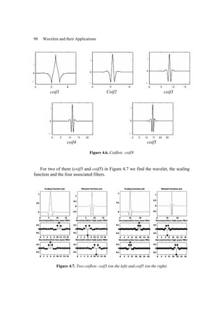
![Wavelet Families 99
As we can see, coiflets, as well as the associated scaling functions, are much
more symmetric than the Daubechies wavelets dbN.
With respect to the length of the support, coifN can be compared to db3N or
sym3N. From the point of view of the number of zero moments of ψ , coifN can be
compared to db2N or sym2N.
The principal interest of coiflets lies in the following property: if f is a
sufficiently regular function, then the approximation coefficient ( )
,
, j k
f ϕ for a
sufficiently large j is estimated well by /2
2 (2 )
j j
f k
− −
, i.e. a sampled value of the
function f . Moreover, if f is a polynomial of a degree equal to 1
N − , the
estimate corresponds to the exact value. This property is used to control the
difference between the development of a given signal on ,
j k
ϕ and a sampled
version of the signal.
4.4.2. Biorthogonal wavelets with compact support: bior
Biorthogonal wavelets extend the families of orthogonal wavelets (see Chapter
2). It is a well-known fact in the filter theory community that symmetry and perfect
reconstruction are incompatible (except for the Haar wavelet) when the same FIR
filters are used for decomposition and for reconstruction process. To circumvent this
difficulty two wavelets are introduced instead of one:
− the first one, ψ , is used for analysis, and the coefficients of a signal s are
( ) ( )
, ,
j k j k
c s x x dx
ψ
= ∫ ;
− the other one, ψ , is used for synthesis: , ,
,
j k j k
j k
s c ψ
= ∑ .
The wavelets ψ and ψ are linked by duality relations:
, ', '
( ) ( ) 0
j k j k
x x dx
ψ ψ =
∫ for '
k k
≠ or '
j j
≠
0, 0, '
( ) ( ) 0
k k
x x dx
ϕ ϕ =
∫ for '
k k
≠
It thus becomes possible to concentrate the properties desirable for analysis (the
number of zero moments for example) in the wavelet ψ , while the properties
interesting for synthesis (regularity, symmetry) can be concentrated in ψ .
Figure 4.8 presents biorthogonal wavelets constructed by Daubechies (see [DAU
92] p. 259 and 262-285). For each of them we find the graphs of the ψ and ψ
functions represented in Figure 4.8.](https://image.slidesharecdn.com/03-misiti-waveletsandtheirapplications-220602130041-0d67589d/85/03-Misiti_-_Wavelets_and_Their_Applications-pdf-121-320.jpg)

![Wavelet Families 101
As we can see, the ψ and ψ functions can have very different regularities. The
wavelets ψ and ψ , as well as the scaling functions ϕ and ϕ , have compact
support generating two dual multi-resolution analyses which enable the use of the
fast Mallat algorithm for calculations. Let us note that wavelets ψ and ψ of
biorNr.Nd have Nr and Nd zero moments respectively.
Let us note, finally, that the roles of the pairs ( , )
ϕ ψ and ( , )
ϕ ψ are symmetric
and that they may therefore be exchanged to obtain another couple of biorthogonal
wavelets.
4.4.3. Orthogonal wavelets with non-compact support
4.4.3.1. The Meyer wavelet: meyr
The meyr wavelet is one of the first wavelets. It was constructed by Meyer in the
mid-1980s (see [DAU 92] p. 117, 119, 137 and 152).
It is an infinitely derivable orthogonal wavelet but it does not have compact
support. The graphs of the ψ and ϕ functions are represented in Figure 4.9.
Figure 4.9. Meyer wavelet: scaling function (on the left) and wavelet (on the right)](https://image.slidesharecdn.com/03-misiti-waveletsandtheirapplications-220602130041-0d67589d/85/03-Misiti_-_Wavelets_and_Their_Applications-pdf-123-320.jpg)
![102 Wavelets and their Applications
The ψ and ϕ functions are both defined in the frequency domain, using an
auxiliary function noted ν :
( )
( )
( )
( )
1/2 /2
1/2 /2
3
(2 ) sin 1
2 2
3
ˆ( ) (2 ) cos 1
2 4
0
i
i
e
e
ω
ω
π
π ν ω
π
π
ψ ω π ν ω
π
−
−
⎧
⎪ −
⎪
⎪
⎪
⎪
⎪
⎪
⎪
= −
⎨
⎪
⎪
⎪
⎪
⎪
⎪
⎪
⎪
⎩
if
if
if
2 4
3 3
4 8
3 3
2 8
,
3 3
π π
ω
π π
ω
π π
ω
≤ ≤
≤ ≤
⎡ ⎤
∉ ⎢ ⎥
⎣ ⎦
where 4 2 3
( ) (35 84 70 20 )
a a a a a
ν = − + − with [ ]
0,1
a ∈ .
( )
( )
1/2
1/2
(2 )
3
ˆ( ) (2 ) cos 1
2 2
0
π
π
ϕ ω π ν ω
π
−
−
⎧
⎪
⎪
⎪
⎪
⎪
⎪
⎪
⎪
= −
⎨
⎪
⎪
⎪
⎪
⎪
⎪
⎪
⎪
⎩
if
if
if
2
3
2 4
3 3
4
3
π
ω
π π
ω
π
ω
≤
≤ ≤
≥
Changing the auxiliary function ν we obtain a family of functions that generate
an orthogonal analysis under certain conditions for ν .
The function ψ is not compactly supported, but when x → ∞ it converges to 0
as in the next formula:
, n
n C
∀ ∈ ∃ such that 2
( ) (1 ) n
n
x C x
ψ −
≤ +
Moreover, ψ is infinitely derivable and the same property of decrease applies to
each of the derivatives. The ψ function is thus rapidly decreasing.
4.4.3.2. An approximation of the Meyer wavelet: dmey
Since the ψ function does not have compact support, it is difficult to use it in
practice because it requires the use of infinite impulse response filters. There are,
nevertheless, FIR approximations of this wavelet enabling fast decomposition (see
[ABR 95] p. 268). In Figure 4.10, in addition to the wavelet, we find the scaling
function and the four associated filters.](https://image.slidesharecdn.com/03-misiti-waveletsandtheirapplications-220602130041-0d67589d/85/03-Misiti_-_Wavelets_and_Their_Applications-pdf-124-320.jpg)
![Wavelet Families 103
Figure 4.10. FIR approximation of the Meyer wavelet
4.4.3.3. Battle and Lemarié wavelets: btlm
The Battle and Lemarié family of wavelets is one of the first and appeared
towards the end of the 1980s. Its construction is based on the spline functions (see
[DAU 92] p. 146-151). In fact, there exist two forms of this wavelet: one providing
an orthogonal analysis, the other not.
For 1
N = the scaling functions are linear splines. For 2
N = the scaling
functions are compactly supported quadratic splines. More generally, for any n,
n ∈N , N , B-splines of degree N are defined by:
1
1/2 /2 sin( /2)
ˆ( ) (2 )
/2
N
i
e κω ω
ϕ ω π ω
ω
+
− ⎡ ⎤
= ∈
⎢ ⎥
⎢ ⎥
⎣ ⎦
where 0
κ = if N is odd and 1
κ = if N is even.](https://image.slidesharecdn.com/03-misiti-waveletsandtheirapplications-220602130041-0d67589d/85/03-Misiti_-_Wavelets_and_Their_Applications-pdf-125-320.jpg)
![104 Wavelets and their Applications
This formula can be used to construct filters. For 2
N M
= or 2 1
N M
= +
the two-scale relation is written as:
1
1
0
( ) 2 (2 1 )
N
j
N
N
j
x C x M j
ϕ ϕ
+
−
+
=
= − − +
∑
This family of wavelets also has the following properties:
− for even (or odd) N , ϕ is symmetric with respect to 1/2
x = (or 0
x = )
and ψ is antisymmetric (or symmetric) with respect to 1/2
x = ;
− the analysis becomes orthogonal if the ϕ and ψ functions are appropriately
transformed. For 1
N = , for example, we write:
( )
( )
( )
( )
2
1/2 1/2
1/2
2 2
4 sin /2
3 (2 )
1 2cos /2
ω
ϕ ω π
ω ω
⊥ −
=
+
;
− the support of ϕ is compact but the supports of ψ and of ϕ⊥
are not.
Nonetheless, the decrease when time goes to infinity is exponential;
− the ψ wavelets are 1
N − times derivable.
4.4.4. Real wavelets without filters
In certain situations the capacity for parsimonious coding is a secondary
objective. The capacity of accurate and local analysis of the functions requires
redundant time and scale analyses. For this reason we discard the requirement of
generating bases and concentrate on wavelets that verify very weak admissibility
conditions. These wavelets do not have an associated scaling function and thus have
no filters, but have the advantage of having an explicit definition formula. We
provide some examples of such wavelets with real values.
4.4.4.1. The Mexican hat: mexh
It is a function proportional to the second derivative of the Gaussian density
function (see [DAU 92] p. 75):
( )
( )( )
2
1/ 4 2 /2
2
1
3
x
x x e
ψ π− −
= −](https://image.slidesharecdn.com/03-misiti-waveletsandtheirapplications-220602130041-0d67589d/85/03-Misiti_-_Wavelets_and_Their_Applications-pdf-126-320.jpg)
![Wavelet Families 105
It oscillates very little as we can see from its graph represented in Figure 4.11.
Figure 4.11. Mexican hat mexh
4.4.4.2. The Morlet wavelet: morl
This function verifies the condition of admissibility only roughly; despite the fact
that it is a standard function (see [DAU 92] p. 76) defined by:
2
/2
( ) cos(5 )
x
x Ce x
ψ −
=
where C is a normalization constant used for the reconstruction.
Its graph is represented in Figure 4.12 and it shows that it oscillates much more
than the Mexican hat.
Figure 4.12. Morlet wavelet: morl](https://image.slidesharecdn.com/03-misiti-waveletsandtheirapplications-220602130041-0d67589d/85/03-Misiti_-_Wavelets_and_Their_Applications-pdf-127-320.jpg)
![106 Wavelets and their Applications
4.4.4.3. Gaussian wavelets: gausN
We may generalize the Mexican hat by introducing the one-parameter family of
Gaussian derivatives. We start with
2
( ) x
p
f x C e−
= and consider the p order
derivative of f sequence p
C so that
2
( ) 1
p
f = . The graph of the 8th
Gaussian
derivative is represented in Figure 4.13.
Figure 4.13. Eighth derivative of a Gaussian function: gaus8
4.4.5. Complex wavelets without filters
In this section we examine some wavelets or wavelet families with complex
values, which can be found in the book by Teolis (see [TEO 98] p. 62-65).
4.4.5.1. Complex Gaussian wavelets: cgau
We can extend the real one-parameter family of Gaussian derivatives to the
complex case. We start with
2
( ) ix x
p
f x C e e
− −
= and consider, as previously, the
order p derivative of f . Here are the real and imaginary parts, the modulus and the
angle of the wavelet of this family for 8
p = .](https://image.slidesharecdn.com/03-misiti-waveletsandtheirapplications-220602130041-0d67589d/85/03-Misiti_-_Wavelets_and_Their_Applications-pdf-128-320.jpg)


![Wavelet Families 111
or, equivalently:
0 1
, 0
j
A A A j
ϕ − −
= = = = = ∀ > and 0 , 0
j
D j
−
= ∀ ≥ .
Consequently, by using successively 0
V , 1
V− ,…, j
V− , etc., we obtain:
0 1
0, ,
1,
j
p p p
p j p
p
p p p
a a a
ϕ ϕ ϕ ϕ
−
−
−
−
∈ ∈ ∈
= = = = =
∑ ∑ ∑
In addition, for a fixed 0
J > the reconstruction phase of the Mallat algorithm
makes it possible to calculate the components of J
A−
using those of 1
J
A− +
and
1
J
D− +
(see relation [3.15] in Chapter 3):
[ ] [ ]
1 1
2 2
J J J
m p p
m p m p
p p
a a LoR d HiR
− − + − +
− −
∈ ∈
= +
∑ ∑
where LoR and HiR are the reconstruction filters associated with the scaling
function and the wavelet. Since the detail 1
J
D− +
is equal to zero:
[ ]
1
2
J J
m p m p
p
a a LoR
− − +
−
∈
= ∑
The process is iterated until level 0, using the fact that all the details are zero.
Ultimately, starting from the sequence { }
0 0
0 1 , 0 , 0
p
a a p
= = ∀ ≠ and
applying the reconstruction phase of the Mallat algorithm with zero components for
details J times, we calculate the sequence { }
J
m
m
a −
. As we shall see in the last
section, the sequence { }
2
2
J J
m
m
a−
is then an “approximation” of the sequence of
values ( )
{ }
2 J
m
m
ϕ −
. For instance, if ϕ is Hölderian of the order α over , the
approximation error is less than 2 J
D α
−
. This means that very good precision is
reached after few iterations, say 10
J = , as in the example in the following section.](https://image.slidesharecdn.com/03-misiti-waveletsandtheirapplications-220602130041-0d67589d/85/03-Misiti_-_Wavelets_and_Their_Applications-pdf-133-320.jpg)


![Chapter 5
Finding and Designing a Wavelet
5.1. Introduction
It is possible that for certain applications we do not find a suitable wavelet
among the known options. It is then natural to try to produce a new wavelet adapted
to the specific problem being treated. In this chapter we are interested in two wavelet
construction processes: one is useful for continuous analysis and the other is linked
to the discrete case.
In the first part of this chapter we consider the construction of wavelets usable
for continuous analysis. This problem does not present great difficulty as the
requirements to obtain such wavelets are relatively limited. We proceed in the
following manner: starting from a pattern which, in general, is not a wavelet, we
seek the wavelet nearest to the given form in the least squares sense. The usefulness
of the construction process is demonstrated when this is applied to a detection
problem. The task consists of employing the adapted wavelet to identify in a signal
the patterns stemming from the basic form via translation and dilation.
In the second part of this chapter we tackle the construction of wavelets for
discrete analyses, which is, in turn, more delicate. Until a few years ago, it was still
only a subject for specialist discussion. Recently, the lifting method developed by
Sweldens (see [SWE 98]) has made this task easier. It makes it possible to construct
an infinite number of biorthogonal wavelet bases starting from a given biorthogonal
wavelet base.](https://image.slidesharecdn.com/03-misiti-waveletsandtheirapplications-220602130041-0d67589d/85/03-Misiti_-_Wavelets_and_Their_Applications-pdf-137-320.jpg)

![Finding and Designing a Wavelet 117
For f in 2
L the existence of the coefficients ( , )
f
C a b is ensured once ψ is in
2
L . Nonetheless, in order to enable the inversion of the transformation, it is
necessary to choose functions ψ belonging to 1 2
L L
∩ and satisfying the following
admissibility condition relating to the Fourier transform ψ̂ of ψ :
( )
2 2
0
0
ˆ ˆ
( ) ( )
-
CNS ad d d
ψ ω ψ ω
ω ω
ω ω
+∞
−∞
= < +∞
∫ ∫ [5.1]
These hypotheses about the ψ function guarantee the possibility of calculating
the inverse transform. We then say that ψ is an admissible wavelet.
To verify that a real function is a wavelet we use the following simpler sufficient
admissibility condition:
( )
-
CS ad ψ real, 1 2
L L
ψ ∈ ∩ , ( )
t t dt
ψ < +∞
∫R
and ( ) 0
t dt
ψ =
∫
The condition ( )
-
CS ad makes it possible to affirm that the Fourier transform
1
ˆ C
ψ ∈ with ( )
ˆ 0 0
ψ = ; consequently, the integrals of the condition ( )
-
CNS ad
exist.
5.2.1.2. Simple examples of admissible wavelets
The admissibility condition and the condition ( )
-
CS ad are very weak and it is
easy to construct wavelets usable for continuous analysis. Almost any function
integrating to zero is appropriate, provided that it also verifies some elementary
properties.
Let us cite some simple examples of ψ functions verifying the condition
( )
-
CS ad .
If f is Gaussian, ( )
2
Bt
f t Ae−
= with A ∈ and 0
B > , then all its
derivatives satisfy the sufficient admissibility condition. Indeed, for all n ∗
∈
there is a polynomial n
P , such that ( )
( ) ( )
2
n Bt
n
f t P t e−
= ; therefore,
( ) 1 2
n
f L L
∈ ∩ , ( ) 1
n
tf L
∈ and ( )
( ) ( )
1
0
n n
f t dt f
+∞
−
−∞
⎡ ⎤
= =
⎣ ⎦
∫ .
More generally, if f belongs to the set of rapidly decreasing functions, all the
derivatives of f satisfy the condition.](https://image.slidesharecdn.com/03-misiti-waveletsandtheirapplications-220602130041-0d67589d/85/03-Misiti_-_Wavelets_and_Their_Applications-pdf-139-320.jpg)
![118 Wavelets and their Applications
Figure 5.1. Gaussian functions: 1st
derivative on the left and 8th
derivative on the right
If ( ) ( )
1 2
f L L
+ +
∈ ∩ with ( )
1
tf L +
∈ , by extending f to −
in an
odd fashion we also obtain a function satisfying the sufficient admissibility
condition. We can, in particular, choose a continuous or piecewise continuous
function f over +
with a compact support, as in the example in Figure 5.2.
Figure 5.2. On the left, a function f defined over +
.
On the right, the wavelet ψ obtained by extension of f
The construction of wavelets with compact support and arbitrary regularity is
easy. Let us consider, for example, the following family with a parametern ∈ :
( ) ( )
[ ] ( )
[ ]
( )
1
-1,1
sgn sin 1
I
n
n
n
f t t t t
π
+
=
The sufficient admissibility condition is satisfied. Moreover, ( )
1
n
n
f C −
∈
and it is zero outside of the segment [ ]
1,1
− .](https://image.slidesharecdn.com/03-misiti-waveletsandtheirapplications-220602130041-0d67589d/85/03-Misiti_-_Wavelets_and_Their_Applications-pdf-140-320.jpg)
![Finding and Designing a Wavelet 119
Figure 5.3. Function 3
f on the left and function 8
f on the right
In order to extend a support equal to [ ]
,
a b we can, for example, consider the
family { }
n
g defined by ( ) ( ) ( )
( )
( )
1
2
1 1
n n
g t f b t a t
= + + − for n ∈ , or
construct an adapted polynomial function.
5.2.1.3. Construction of wavelets approaching a pattern
On the basis of the given function f with compact support and finite energy we
may consider the construction of a wavelet usable for continuous analysis,
approximating this function as well as possible, in the least squares sense. Various
construction methods are possible.
First method
Let us denote by [ ]
,
a b an interval containing the support of f and take a family
{ } 1
N
i i
F ρ =
= of N functions, continuous or piecewise continuous on [ ]
,
a b . Let us
suppose that the family F is linearly independent in ( )
2 ,
L a b .
We want to construct the approximation in the least squares sense of the function
f using a finite linear combination of the form
1
N
i i
i
ψ α ρ
=
= ∑ . Given the
hypotheses on f and F , the approximation ψ clearly satisfies the two conditions
1 2
L L
ψ ∈ ∩ and 1
t L
ψ ∈ . The function ψ must integrate to zero (we can foresee
having other vanishing moments). This condition reduces to the following linear
constraint:
1
0
N
i i
i
R
α
=
=
∑ where ( )
b
i i
a
R t dt
ρ
= ∫ .](https://image.slidesharecdn.com/03-misiti-waveletsandtheirapplications-220602130041-0d67589d/85/03-Misiti_-_Wavelets_and_Their_Applications-pdf-141-320.jpg)
![120 Wavelets and their Applications
The vector { } 1
N
i i
α α =
= and, consequently, the function
1
N
i i
i
ψ α ρ
=
= ∑ are
obtained by solving a linear system. More precisely, by noting:
– G the Gram matrix ( )
x
N N defined by ( ) ( )
b
i j i j
a
G t t dt
ρ ρ
= ∫ ;
– M the matrix of constraints ( )
1xN with i i
M R
= ;
– B the vector ( )
x1
N defined by ( ) ( )
b
i i
a
B f t t dt
ρ
= ∫ ;
the vector α and the Lagrange multiplier λ associated with the constraint are the
solutions of the linear system:
0
0
t B
G M
M
α
λ
⎛ ⎞ ⎛ ⎞
⎛ ⎞
⎟
⎜ ⎟
⎜
⎟
⎜
⎟
⎜ ⎟
⎟ ⎜
=
⎜
⎟ ⎟
⎜ ⎟ ⎜
⎟⎜ ⎟
⎟
⎜ ⎟
⎜ ⎟
⎜
⎜
⎟
⎟⎝ ⎠
⎜ ⎝ ⎠
⎝ ⎠
When the family F is not orthogonal to the set of constants, M becomes the
matrix of a surjective application of N in and the solution is therefore unique.
EXAMPLE 5.1.
In this example we construct two approximating wavelets differing by the choice
of the F functions family. Let us consider the function f with the support [ ]
1,1
− ,
defined by:
( )
[ ]
( )
[ ]
( )
{ } ( )
1 2
0,1 -1,0
1
I 1
I sin
f t C t C t t
π
= +
Let us note that ( )
( )
1 2
2 C C
f t dt
π
−
=
∫ and thus ( ) 0
f t dt ≠
∫ , if
1 2
C C
≠ .
Let us take, for example, 1 1
C = and
1
2 2
C = .
The wavelet represented in the left graph in Figure 5.4 is obtained using the
family of polynomials of degree 2
≤ over the interval [ ]
1,1
− as family F . By
employing as family F the same family of polynomials but on a larger interval,
here [ ]
2,1
− , we obtain the wavelet of the right graph.](https://image.slidesharecdn.com/03-misiti-waveletsandtheirapplications-220602130041-0d67589d/85/03-Misiti_-_Wavelets_and_Their_Applications-pdf-142-320.jpg)
![Finding and Designing a Wavelet 121
Of course, the result does not seem very satisfactory. To improve it, it is
necessary to increase the degree of the F polynomials and to add continuity
constraints to the ψ function. Let us examine that in the next section.
Figure 5.4. Approximation by polynomials of degree 2
≤ :
on the left on [ ]
1,1
− , on the right on [ ]
2,1
−
Second method
Since the family F consists of continuous functions on [ ]
,
a b we may seek a
function ψ continuous on the real line . That amounts to imposing two additional
linear constraints ( ) 0
a
ψ = and ( ) 0
b
ψ = leading to ( )
1
0
N
i i
i
a
α ρ
=
=
∑ and
( )
1
0
N
i i
i
b
α ρ
=
=
∑ .
The constraints matrix M becomes a ( )
3xN matrix defined by:
1, i
i
M R
= , ( )
2, i
i
M a
ρ
= and ( )
3, i
i
M b
ρ
= , 1, ,
i N
∀ =
EXAMPLE 5.2.
Let us again take the function f from the previous example and use the
polynomials of degree 3
≤ on [ ]
1,1
− to construct a wavelet ψ that would be the
approximation of f in the least squares sense. We obtain the approximations
represented in Figure 5.5.
f
f
ψ
ψ](https://image.slidesharecdn.com/03-misiti-waveletsandtheirapplications-220602130041-0d67589d/85/03-Misiti_-_Wavelets_and_Their_Applications-pdf-143-320.jpg)
![122 Wavelets and their Applications
Figure 5.5. Approximation by polynomials of degree 3
≤ on [ ]
1,1
− : on the left
unconstrained, on the right with the constraints ( )
1 0
ψ − = and ( )
1 0
ψ =
Third method
We can use a more direct construction method. We seek the best approximation
of f in the least squares sense, within the space of functions orthogonal to
constants. On the basis of 2
f L
∈ with ( ) [ ]
supp ,
f a b
⊂ , the following ψ function
approximates f and verifies the admissibility condition:
( ) [ ]
,
1
I
b
a b
a
f f
ψ = − ∫
If f is continuous over the interval [ ]
,
a b , satisfying the two additional
constraints ( ) 0
a
ψ = and ( ) 0
b
ψ = leads to seeking a wavelet ψ of the form:
( ) [ ]
2
,
1
I a b
f t t
ψ α β γ
= − + +
The coefficients α, β and γ are calculated solving the linear system:
( )
( )
3 3 2 2
2
2
3 2
1
1
b
a
b a b a
b a f
a a f a
f b
b b
α
β
γ
⎛ ⎞
− − ⎟
⎜ ⎟
− ⎛ ⎞
⎜ ⎟⎛ ⎞ ⎟
⎜ ⎜
⎟ ⎟ ⎟
⎜
⎜ ⎜
⎟ ⎟ ⎟
⎜
⎜ ⎜
⎟ ⎟ ⎟
⎜
⎜ ⎜
⎟ ⎟ ⎟
⎜
⎟
⎜ = ⎜
⎟ ⎟
⎟⎜
⎜ ⎜
⎟ ⎟
⎟⎜
⎜ ⎟ ⎟
⎜
⎟ ⎟
⎜ ⎟
⎜ ⎜
⎟ ⎟
⎟ ⎟
⎜
⎜
⎜ ⎜
⎝ ⎠
⎟ ⎟
⎟ ⎟
⎜
⎜ ⎜
⎝ ⎠
⎟ ⎟
⎜ ⎟
⎟
⎜
⎜ ⎟
⎝ ⎠
⎟
⎜
∫
f f
ψ ψ](https://image.slidesharecdn.com/03-misiti-waveletsandtheirapplications-220602130041-0d67589d/85/03-Misiti_-_Wavelets_and_Their_Applications-pdf-144-320.jpg)
![Finding and Designing a Wavelet 123
Fourth method
In practice and for numerical calculations we generally know only one sampling
of the function f over the [ ]
,
a b interval. We have a finite set of values
( )
{ } 1, ,
,
k k k K
t y =
such that:
k
a t b
≤ ≤ and ( )
k k
y f t
≈ .
As above, we consider a family { } 1
N
i i
F ρ =
= linearly independent in ( )
2 ,
L a b ,
and we denote by V the span vector space of F. Formulated for this finite set of
pairs, the problem amounts to seeking { } 1
N
i i
α α =
= in N
and thus
1
N
i i
i
ψ α ρ
=
= ∑ such that:
2 2
= =
[ ( ) ] [ ( ) ] such that ( ) 0
K
k k β k k β
β
k 1 1
ψ υ
Min
N
K b
a
k
t y t y t dt
υ
∈
⎧ ⎫
− = − =
⎨ ⎬
⎩ ⎭
∑ ∑ ∫
{
where for β in N ,
1
N
i i
i
vβ β ρ
=
= ∑ .
It is thus a problem of minimization in the least squares sense with a constraint, a
problem similar to the one considered previously. The vector α and the Lagrange
multiplier λ associated with the constraint are obtained by solving the linear
system:
0
0
t B
G M
M
α
λ
⎛ ⎞ ⎛ ⎞
⎛ ⎞
⎟
⎜ ⎟
⎜
⎟
⎜
⎟
⎜ ⎟
⎟ ⎜
=
⎜
⎟ ⎟
⎜ ⎟ ⎜
⎟⎜ ⎟
⎟
⎜ ⎟
⎜ ⎟
⎜
⎜
⎟
⎟⎝ ⎠
⎜ ⎝ ⎠
⎝ ⎠
with G , M and B defined by:
( ) ( )
1
K
i j i j
k k
k
G t t
ρ ρ
=
= ∑ , ( )
b
i i
a
M t dt
ρ
= ∫ , ( )
1
K
i i
k k
k
B y t
ρ
=
= ∑ .](https://image.slidesharecdn.com/03-misiti-waveletsandtheirapplications-220602130041-0d67589d/85/03-Misiti_-_Wavelets_and_Their_Applications-pdf-145-320.jpg)
![124 Wavelets and their Applications
5.2.2. Application to pattern detection
In this section we propose considering the following detection problem. We take
S signals consisting of a linear combination of dilations-translations ( )
t b
f
a
−
of a
basic form f and, possibly, also a noise and a “low frequency” function.
In this context, only ( )
S t and ( )
f t are known. We have to identify the number
of patterns
1
K
k
k k
t b
f
a =
⎧ ⎛ ⎞⎫
−
⎪ ⎪
⎪ ⎪
⎟
⎜ ⎟
⎨ ⎬
⎜ ⎟
⎜ ⎟
⎜
⎪ ⎪
⎝ ⎠
⎪ ⎪
⎩ ⎭
and the value of the pairs (scale, position) ( )
{ }
,
k k k
a b .
The following process is used:
– find an acceptable wavelet ψ approximating the form f using one of the
methods presented in the previous section;
– perform an analysis of S using the adapted wavelet ψ ;
– select ( )
,
k k
a b seeking the maxima of the coefficients’ surface.
In this section we will find three increasingly complex examples, for which we
demonstrate that:
– the above process performs well;
– the use of another wavelet systematically leads to worse results.
EXAMPLE 5.3.
Let us consider the basic form already encountered in example 5.1, i.e. the
function f defined by:
( )
[ ]
( )
[ ]
( )
{ } ( )
1 2
0,1 -1,0
1
I 1
I sin
f t C t C t t
π
= +
with 1 1
C = and 2 0.9
C = . Since ( )
( )
2
1 2 0.0637
C C
f t dt π
−
=
∫ 0
≠ , this
form is not a wavelet.
We construct a signal S containing two specimens dilated from this basic form
f and depicted in Figure 5.6.](https://image.slidesharecdn.com/03-misiti-waveletsandtheirapplications-220602130041-0d67589d/85/03-Misiti_-_Wavelets_and_Their_Applications-pdf-146-320.jpg)


![Finding and Designing a Wavelet 127
Figure 5.9. Contour plot of the coefficients of the signal analyzed with the sym4 wavelet
EXAMPLE 5.4.
Let us consider a second example, where we will partially superimpose two
translated and dilated versions of another basic form f , defined by:
( )
[ ]
( )
[ ]
( )
{ } ( )
[ ]
( ) ( )
1 2
0,1 -1,0 -1,1
1
1
I 1
I sin 1
I sin 4
4
f t C t C t t t t
π π
= + +
Figure 5.10. Pattern f and adapted wavelet ψ obtained
using polynomials of degree 6
≤ on [ ]
1,1
−
f
ψ](https://image.slidesharecdn.com/03-misiti-waveletsandtheirapplications-220602130041-0d67589d/85/03-Misiti_-_Wavelets_and_Their_Applications-pdf-149-320.jpg)
![128 Wavelets and their Applications
with 1 1
C = and 2 0.9
C = , and, thus, also here ( )
( )
2
1 2 0.0637
C C
f t dt π
−
=
∫ .
We construct an admissible wavelet approximating f using polynomials of
degree 6
≤ on [–1,1] (see Figure 5.10).
We construct a signal S containing two dilated and partially superimposed
specimens of this basic form.
Figure 5.11. Constructed signal: ( ) ( ) ( )
2
t T t T
S t f f
− −
= +
32 8 , with T = 48
We successively analyze signal S with the adapted wavelet and the db1 wavelet.
(Figures 5.12 and 5.13, respectively). In the two analyses the joint position of the
two dilated forms is clearly detected. Nonetheless, the adapted wavelet is more
accurate in locating the two scales 32 and 8. Compared to the preceding one, the
analysis with db1 presents a considerable downwards shift of these maxima. Let us
stress that the use of a wavelet with larger support is not efficient for the detection of
the position and scale of every form.](https://image.slidesharecdn.com/03-misiti-waveletsandtheirapplications-220602130041-0d67589d/85/03-Misiti_-_Wavelets_and_Their_Applications-pdf-150-320.jpg)


![Finding and Designing a Wavelet 131
Figure 5.16. Signal analysis with the db1 wavelet
Despite the presence of noise, the wavelet adapted to the form remains more
efficient in locating the two characteristic scales 8 and 4. A wavelet that is more
regular than db1 (for example, dbN or symN) smoothes out the effect of the noise.
However, the scales of the two forms are still badly detected.
5.3. Construction of wavelets for discrete analysis
The rest of this chapter is dedicated to the construction of wavelets for discrete
analysis. First of all, we widen the framework passing by the two-channel filter
banks, whose properties are examined. In particular, we determine the conditions
enabling perfect reconstruction. This classical signal processing approach [EST 77]
leads to what is called quadrature mirror filters (QMF) [MIN 85] or also conjugated
mirror filters [SMI 86], which are also often referred to as QMF.
A perfect reconstruction filter bank is known as “biorthogonal” and the
associated filters as biorthogonal. Lightly constraining conditions make it possible to
obtain such filter banks without too much difficulty. With the “lifting” method it is
then possible to construct an infinite number thereof starting from a biorthogonal
bank. Moreover, thanks to the technique known as “polyphase”, we show [DAU 97]
that all the biorthogonal transformations can be decomposed into elementary lifting
steps.](https://image.slidesharecdn.com/03-misiti-waveletsandtheirapplications-220602130041-0d67589d/85/03-Misiti_-_Wavelets_and_Their_Applications-pdf-153-320.jpg)

![Finding and Designing a Wavelet 133
The inputs and outputs are sequences indexed by .
In each channel the input sequence e is filtered using a
h (respectively a
g ) and
then decimated by 2
↓ . This is the analysis part. In order to synthesize we start with
two sequences, insert the zeros (operation noted 2
↑ ), we filter using s
h and s
g
respectively and, finally, sum up to obtain the output sequence s .
The main property necessary for a filter bank is the property of perfect
reconstruction. After a decomposition followed by a reconstruction without any
intermediate operation we want to obtain an output s equal (possibly up to a close
translation) to the value of input e .
What are the relations that must link the four filters a
h , s
h , a
g and s
g in order
to satisfy this property?
5.3.1.2. The perfect reconstruction condition
Let us consider the filter bank in Figure 5.17, for the case where there is no
intermediate step between decomposition and reconstruction. We may then represent
it more concisely using the following figure.
Figure 5.18. Two-channel filter bank (input-output view)
A necessary and sufficient condition (NSC) linking the four filters a
h , s
h , a
g
and s
g to obtain a perfect reconstruction with a translation of d time units is
provided by the theorem [VET 86]1 where the z-transform of a sequence
( )
k k
s s ∈
= is formally defined by ( ) ,
k
k
k
S z s z z
−
∈
= ∈
∑ .
1 See also [MAL 98], p. 260.
e g
h
s s s
= +
[ ][ ]( )
{ }
2 2
s a
h
s h h e
= ∗ ↑ ↓ ∗
[ ][ ]( )
{ }
2 2
g s a
s g g e
= ∗ ↑ ↓ ∗](https://image.slidesharecdn.com/03-misiti-waveletsandtheirapplications-220602130041-0d67589d/85/03-Misiti_-_Wavelets_and_Their_Applications-pdf-155-320.jpg)
![134 Wavelets and their Applications
THEOREM 5.1. (PERFECT RECONSTRUCTION)– let a
h , a
g , s
h , s
g be the
four bank filters of Figure 5.18. Let us note their respective z-transforms as a
H ,
a
G , s
H and s
G .
For a given d ∈ a NCS, such that for every input e the corresponding output
s verifies ( )
d
s T e
= , where ( )
( )
d k d
k
T e e −
= (i.e. the output s is equal to the
input e delayed by d time units), is:
( ) ( ) ( ) ( ) 2 d
s a s a
H z H z G z G z z−
+ = [5.2]
and:
( ) ( ) ( ) ( ) 0
s a s a
H z H z G z G z
− + − = [5.3]
We speak then of a perfect reconstruction and, when 0
d = , we have perfect
reconstruction without translation: s e
= .
Condition [5.3] is called the anti-aliasing condition.
In the following section we present a simple method of constructing four filters
ensuring the perfect reconstruction condition which is then illustrated using three
examples.
5.3.1.3. Construction of perfect reconstruction filter banks
We can exploit the preceding result to determine the four z-transforms: a
H , s
H ,
a
G and s
G . We seek to easily satisfy condition [5.3], so as to express relation [5.2]
more simply. However, for the simplest choices of the additional constraint, the
reconstruction is necessarily carried out with a translation.
First of all, we will seek an immediate solution of equation [5.3]. Let Θ be an
unspecified function (in practice it is a monomial). If a
H , s
H , a
G and s
G are
selected so that:
( ) ( ) ( )
s a
H z z G z
= Θ − and ( ) ( ) ( )
s a
G z z H z
= −Θ − [5.4]](https://image.slidesharecdn.com/03-misiti-waveletsandtheirapplications-220602130041-0d67589d/85/03-Misiti_-_Wavelets_and_Their_Applications-pdf-156-320.jpg)
![Finding and Designing a Wavelet 135
then relation [5.3] is verified automatically. Using this in [5.2] we obtain just one
equation to be satisfied, where there appear only two unknown factors, a
H and s
H :
( )
( ) ( ) ( ) ( ) 2 ,
( )
d
s a s a
z
H z H z H z H z z d
z
−
Θ
− − − = ∈
Θ −
[5.5]
Relation [5.5] is simplified if we choose an even or odd Θ function, which will
be done later on. The pair ( )
,
a s
H H then verifies:
( ) ( ) ( ) ( ) 2 ,
d
s a s a
H z H z H z H z z d
σ −
− − − = ∈ [5.6]
with 1
σ = + if Θ is even and 1
σ = − if Θ is odd.
In [STR 96] (p. 105-109) and articles by Sweldens, causal filters are privileged.
Relation [5.4] with 1
Θ = is retained, i.e.: ( ) ( )
s a
H z G z
= − and ( ) ( )
s a
G z H z
= − − .
Relation [5.6] is then satisfied with 1
σ = + .
The pair ( )
,
a s
G G satisfies similar relations.
If 1
σ = + , the right-hand side of the equality [5.6] is an odd function of z .
This imposes an odd value ford . Reconstruction has to be performed with a
translation, a “delay”. If 1
σ = − , the first member of the equality is an even
function of z and, thus, d necessarily has an even value. In this case we can take
0
d = , i.e. to obtain a reconstruction without translation.
Regardless of the parity of Θ , posing s a
H
X H H
= and by writing
d
H
X z X
= , the equality [5.6] leads to a very simple equation:
( ) ( ) 2
X z X z
+ − = [5.7]
The first member of the above equality is an even function. If we seek X as a
Laurent series, then X involves only odd powers of z , except for a constant term
equal to 1. In other words, we have:
(2 1)
( ) 1 p
p
p
X z a z− +
∈
= + ∑](https://image.slidesharecdn.com/03-misiti-waveletsandtheirapplications-220602130041-0d67589d/85/03-Misiti_-_Wavelets_and_Their_Applications-pdf-157-320.jpg)

![Finding and Designing a Wavelet 137
Lastly, if we seek finite impulse response filters, the functions a
H , s
H , a
G and
s
G are necessarily Laurent polynomials and Θ is a monomial.
5.3.1.4. Examples of perfect reconstruction filter banks
In this section we present three examples of perfect reconstruction filter banks.
First of all, we take a look at the “lazy wavelet”, which is not a wavelet in the
traditional sense of the term. It leads to the simplest possible perfect reconstruction
filter bank: “it does not do anything”. It is, in particular, the ideal candidate to
initialize a lifting process (see section 5.3.2.1).
EXAMPLE 5.6. (THE “LAZY WAVELET”)
Let us introduce the following notation: for p ∈ , ( )
p
δ stands for the sequence
defined by ( )
1
p
p
δ = and ( )
0
p
k
δ = for k p
≠ . The sequence ( )
0
δ is the element
neutral for the convolution and, more generally, for p ∈ , ( )
( )
p
p
b a T a
δ
= ∗ = ,
i.e. k k p
b a −
= .
Let us take ( ) 1
X z = , 0
d = and ( )
z z
Θ = − , which leads to
( ) ( ) 1
H
X z X z
= = . We can factorize H
X in the form ( ) 1
a
H z = and
( ) 1
s
H z = ; we obtain 1
( )
a
G z z−
= and ( )
s
G z z
= . Thus:
( )
0
a
h δ
= , ( )
0
s
h δ
= , ( )
1
a
g δ
= and ( )
1
s
g δ −
=
The convolutions by a
h and s
h simply correspond to the identity. The filters a
g
and s
g carry out translations of 1 and ( 1)
− respectively. How, then, does the filter
bank operate?
Since [ ][ ]( )
{ }
2 2
s a
h
s h h e
= ∗ ↑ ↓ ∗ and [ ][ ]( )
{ }
2 2
g s a
s g g e
= ∗ ↑ ↓ ∗ ,
the analysis part separates the components with an even index from those with an
odd index, then performs a translation by 1 to the right for the components with an
odd index. According to Figure 5.17 it is illustrated by:
{ }
{ } [ ]
{ }
{ } [ ] { }
1
2
2
2 1
1 2
Id
p
k k p
k k
p
k k
T p
e e
e e
e e
↓
∈ ∈
∈
−
− ∈ ↓ ∈
⎯⎯⎯
→ ⎯⎯⎯
→
= →
⎯⎯⎯
→ ⎯⎯⎯
→](https://image.slidesharecdn.com/03-misiti-waveletsandtheirapplications-220602130041-0d67589d/85/03-Misiti_-_Wavelets_and_Their_Applications-pdf-159-320.jpg)
![138 Wavelets and their Applications
The synthesis part inserts zeros, translates the odd index components by a step of
1 to the left and then calculates the sum:
{ } [ ]
{ } { }
{ } [ ]
{ } { }
1
2
0 0
2
2 1 1 1 1
2
,0, ,0, ,0, ,0,
,0, ,0, , ,0, ,
Id
p p
p T
p
e e e
e
e e e e
−
↑
∈ ⊕
− − −
↑
∈
⎯⎯⎯
→ ⎯⎯⎯
→
⎯⎯⎯
→
⎯⎯⎯
→ ⎯⎯⎯
→
Thus, we find the original sequence.
EXAMPLE 5.7. (“HAAR FILTERS”)
The second example deals with the simplest orthogonal wavelet: the Haar
wavelet. A direct application of the preceding algorithm makes it possible to build
the filters associated with this wavelet, but also other filters ensuring perfect
reconstruction but not leading to a wavelet.
Let us take ( ) ( )
1 1
2 2
2 1
1 1
2 2
( ) 2
X z z z z z
− −
= + = + + , 0
d = and
1
( )
z z−
Θ = − .
A first factorization of H
X X
= is given by a s
H
X H H
= with:
( )
1
2
( ) 1
a
H z z
= + and ( )
1
1
2
( ) 1
s
H z z−
= + .
From it we deduce that: ( )
1
2
( ) 1
a
G z z
= − + and ( )
1
1
2
( ) 1
s
G z z−
= − + .
We recognize the z-transforms of the Haar filters:
( ) ( )
( )
0 1
1
2
a
h δ δ −
= + , ( ) ( )
( )
0 1
1
2
s
h δ δ
= +
( ) ( )
( )
0 1
1
2
a
g δ δ −
= − + , ( ) ( )
( )
0 1
1
2
s
g δ δ
= − +
These filters are associated with the Haar scaling function and the Haar wavelet
(see Chapter 4).](https://image.slidesharecdn.com/03-misiti-waveletsandtheirapplications-220602130041-0d67589d/85/03-Misiti_-_Wavelets_and_Their_Applications-pdf-160-320.jpg)

![140 Wavelets and their Applications
5.3.2. Lifting
5.3.2.1. The lifting method
In this section we demonstrate that by using a quadruplet solution of the system
[5.2] and [5.3], we can build an infinite number of other solutions through a method
called “lifting” introduced by Sweldens ([SWE 98], see also [STR 96] p. 214).
The technique is as follows. We start with an odd or even Θ (thus, 1
σ = ± ),
with d ∈ and two pairs ( )
,
a s
H H and ( )
,
a s
G G that are solutions of [5.4]. Due
to relation [5.6], these pairs are solutions of equation:
( ) ( ) ( ) ( ) 2 d
s a s a
F z F z F z F z z
σ −
− − − = [5.8]
where a
F and s
F are the unknown factors.
The key to lifting is that on the basis of a pair ( )
,
a s
F F , which is a solution of
the previous equation, we can build an infinite number of other solution pairs.
Indeed, let us fix s
F and take a function η . We can define
( ) ( ) ( ) ( )
N
a a s
F z F z F z z
η
= + − (the N exponent stands for “new” and this
convention applies to the rest of the chapter). When 1
σ = and η is even, the pair
( )
,
N
a s
F F is also the solution of [5.8]. We thus produce an infinite number of
solutions parameterized by η . We have the same result for 1
σ = − and an odd η .
If we only consider polynomial solutions, it suffices to take an unspecified
Laurent polynomial P and to take ( )
2
( )
z P z
η = for 1
σ = or ( )
2
( )
z zP z
η =
for 1
σ = − .
By symmetry, if we fix a
F , all the solutions ( )
, N
a s
F F of [5.8] are obtained in a
similar way (this operation is sometimes called dual lifting).
Theorem 5.2 synthesizes the above idea and provides a parameterization of the
infinite number of polynomial quadruplets that solve the system [5.4] and [5.5] (and
thus, also the system [5.2] and [5.3]) obtained by lifting starting from a quadruplet
polynomial solution ( )
, , ,
a a s s
H G H G .](https://image.slidesharecdn.com/03-misiti-waveletsandtheirapplications-220602130041-0d67589d/85/03-Misiti_-_Wavelets_and_Their_Applications-pdf-162-320.jpg)
![Finding and Designing a Wavelet 141
THEOREM 5.2. (PARAMETRIZATION SETTING OF THE SOLUTIONS)3
Primal lifting: let ( )
, , ,
a a s s
H G H G be a polynomial quadruplet verifying [5.4]
and [5.5]. The set of solutions ( )
, , ,
N N
a a s s
H G H G of [5.4] and [5.5] is provided by:
2
2
( ) ( ) ( ) ( )
( ) ( ) ( ) ( )
N
a a a
N
s s s
H z H z G z S z
G z G z H z S z
= +
= −
where S is an unspecified Laurent polynomial.
Dual lifting: let ( )
, , ,
a a s s
H G H G be a polynomial quadruplet verifying [5.4]
and [5.5]. The set of quadruplets ( )
, , ,
N N
a a s s
H G H G solving [5.4] and [5.5] is
yielded by:
2
2
( ) ( ) ( ) ( )
( ) ( ) ( ) ( )
N
s s s
N
a a a
H z H z G z T z
G z G z H z T z
= +
= −
where T is an unspecified Laurent polynomial.
Dual lifting is achieved by exchanging the roles of the “a ” and “s ” indices in
the primal lifting.
5.3.2.2. Lifting and the polyphase method
Up to now we could construct an infinite number of quadruplets with perfect
reconstruction using just one of them thanks to the above parametrization. In fact,
the situation is simpler than it appears. On the basis of elementary quadruplets, for
example of the “lazy wavelet” or the Haar filters (see examples 5.6 and 5.7) we can
obtain an infinite number of solutions by using elementary lifting steps. To specify
this result and to define the concept, a detour to introduce the polyphase method,
which is interesting in itself, is necessary. We thus first describe it in this section and
then examine its consequences for lifting.
In the decomposition part of the filter bank schematized in Figure 5.19 we
perform convolution, followed by decimation where only even index terms are
preserved for each “branch”, also referred to as phase. The odd index terms are not
used. We may wonder about the possibility of permuting the decimation and
filtering so as to make calculation more efficient. It is the object of the polyphase
method.
3 The theorem can also be written using the Fourier transform or directly in the time domain:
[STR 96] p. 216.](https://image.slidesharecdn.com/03-misiti-waveletsandtheirapplications-220602130041-0d67589d/85/03-Misiti_-_Wavelets_and_Their_Applications-pdf-163-320.jpg)

2 a
u h e
= ↓ ∗ , but
( ) [ ]
a a
k n
k n
n
h e e h
−
∈
∗ = ∑ and, thus:
( ) [ ]
2 2
a a
k n
k k n
n
u h e e h
−
∈
= ∗ = ∑ [5.9]
The polyphase method consists simply of reformulating the preceding result by
introducing two elementary sequences: the sequence of even index components and
the sequence of odd index components both for the input and the filter. For a
sequence { }
k k
r r ∈
= let us define the “even” and “odd” sub-sequences by
{ }
2n
P n
r r ∈
= and { }
2 1
n
I n
r r + ∈
= 4. On the basis of [5.9] the new expression
becomes:
[ ] [ ] [ ]
( )
[ ] ( )
( )
[ ]
[ ] [ ]( )
( ) [ ]
( )
2 2 1
2 2 2 2 (2 1)
2 2 1
2 2 1 1
, 1 ,
, ,
1
a a a
n j j
k k n k j k j
n j j
a a
j j
k j k j
j j
a
P I k j a I
P
k j j j
j j
a a
P I
P I
k k
u e h e h e h
e h e h
e h e h
e h T e h
+
− − − +
∈ ∈ ∈
+
− − − +
∈ ∈
− −
−
∈ ∈
= = +
= +
⎡ ⎤
⎡ ⎤
= + ⎢ ⎥
⎣ ⎦ ⎣ ⎦
= ∗ + ∗
∑ ∑ ∑
∑ ∑
∑ ∑
4 If R , P
R and I
R indicate the z-transforms of the sets r , P
r and I
r respectively, then:
( ) ( ) ( )
2 1 2
P I
R z R z z R z
−
= + . Consequently:
( )
( ) ( )
2
2
P
R z R z
R z
+ −
= and ( )
( ) ( )
2
1
2
I
R z R z
R z
z−
− −
= .
u
v
e
a
h 2
↓
a
g 2
↓](https://image.slidesharecdn.com/03-misiti-waveletsandtheirapplications-220602130041-0d67589d/85/03-Misiti_-_Wavelets_and_Their_Applications-pdf-164-320.jpg)
![Finding and Designing a Wavelet 143
Consequently: ( ) [ ]
, ,
1
a a
P I
P I
u e h T e h
= ∗ + ∗ , where 1
T is the operator of
translation of 1 step in time. Similarly we have: ( ) [ ]
, ,
1
a a
P I
P I
v e g T e g
= ∗ + ∗ .
By taking the z-transform of the two previous expressions, we obtain:
1
, ,
1
, ,
( ) ( ) ( ) ( ) ( )
( ) ( ) ( ) ( ) ( )
a P P a I I
a P P a I I
U z H z E z z H z E z
V z G z E z z G z E z
−
−
= +
= +
which is, in matrix form:
, ,
1
, ,
( )
( ) ( ) ( )
( ) ( ) ( ) ( )
P
a P a I
a P a I I
E z
U z H z H z
V z G z G z z E z
−
⎛ ⎞
⎛ ⎞ ⎛ ⎞ ⎟
⎜
⎟ ⎟
⎜ ⎜ ⎟
⎟ ⎟⎜
⎜ ⎜
= ⎟
⎟ ⎟⎜
⎜ ⎜ ⎟
⎟ ⎟⎜
⎜ ⎜ ⎟
⎟ ⎟
⎜ ⎜
⎟ ⎟ ⎟
⎜
⎝ ⎠ ⎝ ⎠⎜
⎝ ⎠
revealing what is called the polyphase analysis matrix5:
, ,
, ,
( ) ( )
( )
( ) ( )
a P a I
Poly
a
a P a I
H z H z
M z
G z G z
⎛ ⎞
⎟
⎜ ⎟
⎜
= ⎟
⎜ ⎟
⎜ ⎟
⎜ ⎟
⎝ ⎠
The analysis part of the diagram can then be illustrated as in Figure 5.20.
Figure 5.20. The polyphase form of the decomposition part of the filter bank.
Id is the identity transformation and T1 is the operator of translation of 1 step in time
5 Some authors call the polyphase matrix the transposition of the matrix used here.
2
↓
e
v
1
T
Poly
a
M
2
↓
u
Id](https://image.slidesharecdn.com/03-misiti-waveletsandtheirapplications-220602130041-0d67589d/85/03-Misiti_-_Wavelets_and_Their_Applications-pdf-165-320.jpg)
![144 Wavelets and their Applications
Thus, we first separate the input e components with an even index P
e from
those with an odd index I
e ; then, the outputs u and v are obtained using
convolutions by filters, ( )
, ,
,
a P a I
h h for example, twice shorter than in Figure 5.19,
and a summation. Thus, there are roughly half as many operations than in the initial
notation, since the terms ,
a
P P
e h
∗ and [ ] ,
1 a
I I
T e h
∗ involved in the calculation of
( ) [ ]
, ,
1
a a
P I
P I
u e h T e h
= ∗ + ∗ are each four times shorter than a
e h
∗ .
Proceeding in a similar way and defining the polyphase synthesis matrix by:
, ,
, ,
( ) ( )
( )
( ) ( )
s P s I
Poly
s
s P s I
H z H z
M z
G z G z
⎛ ⎞
⎟
⎜ ⎟
⎜
= ⎟
⎜ ⎟
⎜ ⎟
⎜ ⎟
⎝ ⎠
the synthesis part can be put in the form represented by Figure 5.21.
Figure 5.21. Polyphase form of the reconstruction part of the filter bank
The perfect reconstruction condition (for 0
d = ) is then rewritten as:
( )
1 0
( ) ( )
0
t
Poly Poly
s a
M z M z
z
⎛ ⎞
⎟
⎜ ⎟
⎜
= ⎟
⎜ ⎟
⎟
⎜
⎝ ⎠
NOTE 5.2.– let us note ( ) ( )
1
a a
H z H z−
= and
Poly
a
M the polyphase matrix
associated with a
H . This amounts to considering a
h the inverse filter of the a
h
filter. We then find a traditional formulation of the previous perfect reconstruction
condition:
( ) 1
( ) ( )
t Poly
Poly
s a
M z M z Id
− =
2
↑
2
↑
s
u
v 1
T
( )
t
Poly
s
M
Id](https://image.slidesharecdn.com/03-misiti-waveletsandtheirapplications-220602130041-0d67589d/85/03-Misiti_-_Wavelets_and_Their_Applications-pdf-166-320.jpg)
![Finding and Designing a Wavelet 145
Apart from the advantages concerning the implementation of the decomposition
and reconstruction algorithms brought by the polyphase method, we also achieve a
particularly important theoretical result.
In the polyphase formulation we may reinterpret the passing from a
( )
, , ,
a a s s
H G H G solution of [5.4] and [5.5] to a new solution ( )
, , ,
N N
a a s s
H G H G
or ( )
, , ,
N N
a a s s
H G H G using theorem [5.2] and multiplying the left side (or the
right) of the polyphase analysis matrix (or of the transpose of polyphase synthesis
matrix) by the matrix:
( )
1
0 1
S z
⎛ ⎞
⎟
⎜ ⎟
⎜ ⎟
⎜ ⎟
⎟
⎜
⎜
⎝ ⎠
or
( )
1 0
1
T z
⎛ ⎞
⎟
⎜ ⎟
⎜ ⎟
⎜ ⎟
⎟
⎜
⎜
⎝ ⎠
(
( )
1
0 1
S z
−
⎛ ⎞
⎟
⎜ ⎟
⎜ ⎟
⎜ ⎟
⎟
⎜
⎜
⎝ ⎠
or
( )
1 0
1
T z
⎛ ⎞
⎟
⎜ ⎟
⎜ ⎟
⎜ ⎟
− ⎟
⎜
⎜
⎝ ⎠
respectively).
Such an operation is called an elementary lifting step.
The factorization theorem 5.3 introduced by Daubechies and Sweldens6 shows
that all quadruplet perfect reconstruction filters have a polyphase matrix that can be
factorized into a sequence of elementary lifting steps.
THEOREM 5.3. (FACTORIZATION)– let there be ( )
, , ,
a a s s
H G H G verifying
[5.4] and [5.5], such that the determinant of the polyphase matrix is equal to 1.
Then, there exist two families of m Laurent polynomials { } 1
m
i i
S =
and { } 1
m
i i
T =
and a constant 0
K ≠ such that the polyphase analysis matrix admits the following
factorization:
( )
( )
1
0
1 0
1
( )
1
1
0 1 0
m
i
Poly
a
i i
K
S z
M z
T z
K
=
⎛ ⎞
⎧ ⎛ ⎞ ⎫
⎛ ⎞
⎪ ⎪ ⎟
⎜
⎟ ⎟
⎜ ⎜
⎪ ⎪ ⎟
⎟ ⎜
⎟
⎜ ⎜
= ⎟
⎨ ⎬
⎟ ⎟ ⎜
⎜ ⎜ ⎟
⎟ ⎟
⎪ ⎪⎜
⎟
⎟⎜
⎜
⎜ ⎜ ⎟
⎟
⎜
⎝ ⎠
⎝ ⎠ ⎝ ⎠
⎪ ⎪
⎩ ⎭
∏
This theorem indicates how to construct an infinite number of solutions of [5.4]
and [5.5] using only elementary lifting steps starting from a perfect reconstruction
quadruplet.
6 This theorem is cited in the article of Daubechies and Sweldens, “Factoring Wavelet
Transform into Lifting Steps” [DAU 97]. See also theorem 7.13 on p. 275 of [MAL 98]](https://image.slidesharecdn.com/03-misiti-waveletsandtheirapplications-220602130041-0d67589d/85/03-Misiti_-_Wavelets_and_Their_Applications-pdf-167-320.jpg)
![146 Wavelets and their Applications
Let us stress that the elementary lifting matrices are explicitly invertible and the
inverses are also elementary lifting matrices, since:
( ) ( )
1
1 1
0 1 0 1
F z F z
− −
⎛ ⎞ ⎛ ⎞
⎟ ⎟
⎜ ⎜
⎟ ⎟
⎜ ⎜
=
⎟ ⎟
⎜ ⎜
⎟ ⎟
⎟ ⎟
⎜ ⎜
⎜ ⎜
⎝ ⎠ ⎝ ⎠
and
( ) ( )
1
1 0 1 0
1 1
F z F z
−
⎛ ⎞ ⎛ ⎞
⎟ ⎟
⎜ ⎜
⎟ ⎟
⎜ ⎜
=
⎟ ⎟
⎜ ⎜
⎟ ⎟
−
⎟ ⎟
⎜ ⎜
⎜ ⎜
⎝ ⎠ ⎝ ⎠
This result has an important algorithmic consequence when a “polyphase”
version of the wavelet decomposition is implemented: calculation of the synthesis
step, the inverse of the preceding step, becomes elementary.
5.3.3. Lifting and biorthogonal wavelets
We can show7 that if ( a
h a
g s
h , s
g ) is a perfect reconstruction filter bank and if
the modulus of the Fourier transforms are bounded, then the families
( ) ( )
{ }
2 , 2
a a k
h k g k ∈
⋅ − ⋅ − and ( ) ( )
{ }
2 , 2
s s k
h k g k ∈
⋅ − ⋅ − are biorthogonal
bases of 2
( )
l . In the particular case where ( a
h , a
g ) = ( s
h , s
g ) we obtain an
orthogonal basis of 2
( )
l .
Let us consider a perfect reconstruction filter bank a
h , s
h , a
g and s
g . If a
h
and s
h have finite length, then:
( )
1
1
( ) ( )
2
2
a a n
n
h
ω
ϕ ω
∞
=
= ∏ and ( )
1
1
( ) ( )
2
2
s s n
n
h
ω
ϕ ω
∞
=
= ∏
converge in ( )
'
S , the set of tempered distributions.
Consequently, a
ϕ and s
ϕ are also defined in ( )
'
S . However, a priori there is
no reason for a
ϕ and s
ϕ to be elements of ( )
2
L . For that to be true, it is
necessary to impose additional conditions. Unfortunately, they are technical and in
general difficult to verify. However, we state the theorem introduced by Cohen
([COH 90] and [MAL 98] p. 265).
7 See theorem 7.9 in [MAL 98] p. 262.](https://image.slidesharecdn.com/03-misiti-waveletsandtheirapplications-220602130041-0d67589d/85/03-Misiti_-_Wavelets_and_Their_Applications-pdf-168-320.jpg)

![148 Wavelets and their Applications
1 1
0 0 0 0
2 2
( ) ( ) ( ) ( ) 1
m m m m
ω ω ω ω
+ + + =
These conditions are well known (see Chapter 2) and simpler to verify.
We can then use the results of lifting in the context of biorthogonal wavelets. Let
us consider the quadruplet ( )
, , ,
a a s s
ϕ ψ ϕ ψ of scaling functions and biorthogonal
wavelets. The process below shows that by using the results of lifting we can
construct others quadruplets of scaling functions and biorthogonal wavelets. This is
“formal”, in the sense that the functions obtained do not necessarily belong to 2
L .
Lifting process8. Let { }
k k
σ ∈
be a family of real numbers containing a finite
number of non-zero elements and ( )
, , ,
a a s s
ϕ ψ ϕ ψ be a quadruplet of scaling
functions and biorthogonal wavelets. For a fixed s
ϕ the family ( )
, , ,
N N N
a a s s
ϕ ψ ϕ ψ ,
defined below, is also “formally” a quadruplet of scaling functions and biorthogonal
wavelets.
( ) ( ) ( )
( ) ( ) ( ) ( )
( ) ( ) ( )
2 2
2 2
N
s s s
k
k
N N N
a a a a
k k
k k
N N
a a a
k
k
x x x k
x h x k x k
x g x k
ψ ψ σ ϕ
ϕ ϕ σ ψ
ψ ϕ
∈
−
∈ ∈
∈
⎧
⎪
⎪ = − −
⎪
⎪
⎪
⎪
⎪
⎪
⎪ = − + −
⎨
⎪
⎪
⎪
⎪
⎪ = −
⎪
⎪
⎪
⎩
⎪
∑
∑ ∑
∑
[5.10]
If we put in parallel the above result and the lifting theorem [5.2], the
modifications to the scaling functions and the wavelets for the associated filters
correspond to a primal lifting of the Laurent polynomial ( )
k
k
k
S z z
σ −
= ∑ .
Let us also note that the new wavelet N
a
ψ verifies the same two-scale relation as
the wavelet a
ψ . The functions N
a
ϕ and N
s
ψ satisfy new two-scale relations taking
into account the contribution of the Laurent polynomial.
8 See Sweldens, “The lifting scheme: a custom-design construction of biorthogonal
wavelets”, Appl. Comput. Harmon. Anal., vol. 3, no. 2, p. 186-200, 1996. See also theorem
7.12 in [MAL 98], p. 273.](https://image.slidesharecdn.com/03-misiti-waveletsandtheirapplications-220602130041-0d67589d/85/03-Misiti_-_Wavelets_and_Their_Applications-pdf-170-320.jpg)
![Finding and Designing a Wavelet 149
Similarly, permuting the roles of a and s in [5.10] on the basis of the same
initial quadruplet ( )
, , ,
a a s s
ϕ ψ ϕ ψ , we also construct quadruplets in the form of
( )
, , ,
N N N
a a s s
ϕ ψ ϕ ψ .
5.3.4. Construction examples
The end of this chapter presents applications of lifting. First we treat examples
that enable us to illustrate the effects of one or more lifting steps and of a
parameterized lifting. Then we outline a lifting solution for two problems:
construction of a wavelet admitting more vanishing moments that the initial wavelet
and then the approximation of a pattern.
The scaling functions and wavelets are constructed using the cascade algorithm
described in Chapter 4.
5.3.4.1. Illustrations of lifting
The four following examples illustrate lifting.
EXAMPLE 5.9. (THE BIOR1.3 WAVELET)
In this example we show how to obtain the bior1.3 wavelet (see Chapter 4) using
lifting.
We start with Haar filters ( )
,
a a
h g and ( )
,
s s
h g whose z-transforms are given
by:
( )
1
2
( ) 1
a
H z z
= + , ( )
1
1
2
( ) 1
s
H z z−
= + ,
( )
1
2
( ) 1
a
G z z
= − + and ( )
1
1
2
( ) 1
s
G z z−
= − + .
The two pairs (scaling function, wavelet) ( )
,
a a
ϕ ψ and ( )
,
s s
ϕ ψ are represented
in Figure 5.22.](https://image.slidesharecdn.com/03-misiti-waveletsandtheirapplications-220602130041-0d67589d/85/03-Misiti_-_Wavelets_and_Their_Applications-pdf-171-320.jpg)


![156 Wavelets and their Applications
an intermediate result. We can also use the split
( )
{ } ( )
{ }
1 1
1 1
( ) 16
32 32
T z z z z z
− −
= − + + + − + leading to a new pair of
biorthogonal wavelets. In Figure 5.30, we illustrate this last construction.
Figure 5.30. The two pairs (scaling function, wavelet) after the 2nd
lifting step
5.3.4.2. Construction of wavelets with more vanishing moments
On the basis of a quadruplet ( )
, , ,
a a s s
ϕ ψ ϕ ψ we wish to construct a wavelet
N
s
ψ that has more vanishing moments than s
ψ . Let us again take the first of the
relations [5.10]: ( )
N
s s s
k
k
x k
ψ ψ σ ϕ
∈
= − −
∑
Z
. We multiply it by m
x , for
0, ,
m M
= and integrate over . The finite family of coefficients { }
k k
σ ∈
satisfies a linear system of ( )
1
M + equations:
( ) ( ) ( ) , 0, ,
m N m m
s s s
k
k
x x dx x x dx x x k dx m M
ψ ψ σ ϕ
∈
= − − =
∑
∫ ∫ ∫
It is therefore enough to find a family of ( )
1
M + coefficients { }
K M
k K
σ
+
leading to a linear system of ( )
1
M + equations with ( )
1
M + unknowns.](https://image.slidesharecdn.com/03-misiti-waveletsandtheirapplications-220602130041-0d67589d/85/03-Misiti_-_Wavelets_and_Their_Applications-pdf-178-320.jpg)
![Finding and Designing a Wavelet 157
Let us consider an elementary example. We start with the quadruplet
( )
, , ,
a a s s
ϕ ψ ϕ ψ , consisting of the scaling function and the Haar wavelet for analysis
and synthesis and we wish to construct a new wavelet N
s
ψ with two vanishing
moments. The new wavelet N
s
ψ has the form:
( ) ( ) ( ) ( )
0 1 1
N
s s s s
x x x x
ψ ψ σ ϕ σ ϕ
= − − −
The numbers 0
σ and 1
σ are solutions of a linear system of two equations with
two unknowns. Since s
ψ has one vanishing moment and s
ϕ integrates 1, the first
equation is reduced to: 0 1
0 σ σ
= + . The calculation of the moments of order 1
yields the second equation:
1
0 1
2
3
σ σ
= + . Consequently,
1
1 4
σ = and
1
0 4
σ = − .
The obtained N
s
ψ function is:
The functions of the new quadruplet are those obtained in the first row of Figure
5.27, from left to right: s
ϕ , N
s
ψ , N
a
ϕ and N
a
ψ .
5.3.4.3. Approximation of a form by lifting
In this section we outline the search for a wavelet approximating a form f by
lifting. We use the first relation of [5.10] to approximate f by
( ) ( ) ( )
N
k
k
x x x k
ψ ψ σ ϕ
∈
= − −
∑
Z
, where the choice of the family ( )
k k
σ ∈Z
is to
be made for given ψ and ϕ .
Let us, firstly, make two observations:
– N
ψ is constructed by “correcting” ( )
x
ψ , which is a fixed function of 0
W ,
using a chosen function belonging to 0
V ;
( )
[ ]
[ ]
[ ]
1
3
2
4
1
5
2
4
1
4
0
0,
,1
1,2
otherwise
N
s
over
over
x
over
ψ
−
⎧
⎪
⎪
⎪
⎪
⎪
⎪
⎪
⎪
= ⎨
⎪
⎪
⎪
⎪
⎪
⎪
⎪
⎩
⎪](https://image.slidesharecdn.com/03-misiti-waveletsandtheirapplications-220602130041-0d67589d/85/03-Misiti_-_Wavelets_and_Their_Applications-pdf-179-320.jpg)
![158 Wavelets and their Applications
– for N
ψ to be a wavelet, its integral has to be zero and, therefore, that
0
k
k
σ
∈
=
∑
Z
.
The approximation of the form f amounts to minimizing 2
N
L
f ψ
− , i.e. to
minimizing the sum of the two terms:
( ) ( ) ( )
( ) ( ) ( )
2
0 0
0 0
2
2
2
N
V V k
L
k
V V k
k
f f P f P f x k
f P f P f x k
ψ ψ σ ϕ
ψ σ ϕ
⎛ ⎞
⎟
⎜
− = − + − − − ⎟
⎜ ⎟
⎟
⎜
⎝ ⎠
= − − + + −
∑
∑
because ( )
0
V
f P f
− is orthogonal to 0
V , 0 0
W V
ψ ∈ ⊥ therefore,
( )
0
0
W
f P f V
ψ
− − ⊥ and ( ) ( )
0
0
V k
P f k V
σ ϕ
+ ⋅ − ∈
∑ .
The first term is fixed when ψ is fixed and the lifting only makes it possible to
minimize the second term.
It is important to note that the corrections are on the same scale as f . An
approach consists of dilating f so that the scale of the corrections becomes small
compared to that of the approximated form. The technique would then consist of
approximating a dilated version of f , ( ) ( )
2
2 2
j
j
j
F x f x
−
−
− = for 0
j > by its
projection onto 0
V and then contracting the obtained function. The result is
obviously better because this amounts to approximating f by its projection onto
j
V− , which is a space providing finer approximations. Indeed, for the example of
the Haar wavelet, 0
V consists of functions constant in the intervals [ , 1[
k k + ,
k ∈ Z , whereas j
V− is the space of functions constant in 2j
times smaller
intervals [k2–j
, (k + 1) 2–j
[. This approach has been deeply investigated by Mesa
[MES 05].](https://image.slidesharecdn.com/03-misiti-waveletsandtheirapplications-220602130041-0d67589d/85/03-Misiti_-_Wavelets_and_Their_Applications-pdf-180-320.jpg)
![Chapter 6
A Short 1D Illustrated Handbook
6.1. Introduction
Interesting signals generally exhibit numerous non-stationary characteristics that
constitute a considerable part of the information contained in a series: drifts, trends,
breakdowns, beginnings and ends of events, transitory phenomena. Most classical
mathematical approaches widely used are well adapted to the study of stationary
processes. Among others we may cite the spectral approach linked to the Fourier
transform and that resulting from the ARMA processes [AZE 84].
This chapter takes you through the wavelet decomposition of signals and
compiles “illustrated handbooks” associated with classical situations frequently
encountered in statistics or signal processing. Its application is pedagogical as well
as practical, and is based on the analysis of several elementary examples to learn
how to recognize forms. The signals are presented followed by tests and trials, and
we comment on the results. This chapter consists of three parts.
The first part1, which is also the longest, concerns discrete signal analysis. It is
intentionally over-detailed and exploits the capacity of wavelets to decompose a
signal into a sum of approximation and detail signals. The topics dealt with relate to
the identification of trends, periodic signals, noises, breakdowns and discontinuities.
The commented analysis of 10 simulated signals constitutes the first “illustrated
handbook”. It is supplemented by an examination of two real signals: an electrical
load curve and an electroencephalogram.
1 This part has borrowed much from the article [MIS 93] published in Revue de Statistique
Appliquée, which the authors thank for the kind authorization.](https://image.slidesharecdn.com/03-misiti-waveletsandtheirapplications-220602130041-0d67589d/85/03-Misiti_-_Wavelets_and_Their_Applications-pdf-181-320.jpg)


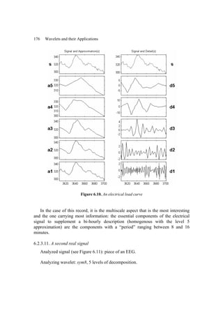

![178 Wavelets and their Applications
The examination of approximations, from the finest 1
A to the coarsest 5
A , leads
to observing that passing from level 3 to level 4 causes the clearest break. This
confirms the importance of the detail at level 4 since 4 3 4
A A D
− = .
Details at levels 1 and 2 primarily capture the local irregularities caused by noise
and the abrupt changes of the signal at the positions 80, 620 and 730.
Detail 4
D isolates the two areas sought in this analysis (see boxes appearing in
detail 4). They correspond to zones locally homogenous in frequency and of
considerable amplitude.
Wavelet analysis makes it possible to easily capture useful information in level 4
detail that we could then process and analyze.
6.3. The contribution of analysis by wavelet packets
Wavelet packets are a generalization of orthogonal wavelets. They enable a finer
analysis by decomposing not only the approximation but also the detail at each level.
Introduced to deal with the lack of frequency resolution in the wavelet analysis, their
principle is to some extent to cut the details up in frequency bands (see Chapter 2).
Consequently, we construct representations of coefficients in the time-frequency
plane that are adequate to highlight their contribution.
Here we illustrate the improvement brought by wavelet packets for the frequency
resolution of the analysis with three examples: two chirps (linear and quadratic)
followed by a periodic signal and finally, in the last example, we consider a more
composite signal.
6.3.1. Example 1: linear and quadratic chirp
The first signal presented is a “linear chirp”, i.e. an oscillating signal whose
frequency 250 t
π increases linearly with time.
We consider the function ( ) [ ]
2
sin 250 , 0,1
y t t
π
= ∈ and take a sampling of
length 512. In Figure 6.12 we present an analysis at level 4 by wavelets (on the left)
and by wavelet packets (on the right) using the wavelet db2.
Decomposition by wavelets (stemming from the analysis by packets) and
complete decomposition by wavelet packets are represented in the same way. The
horizontal bands associated with the packets are arranged in order of ascending
frequency, lower frequencies being at the bottom. The coefficients are colored
according to their absolute value.](https://image.slidesharecdn.com/03-misiti-waveletsandtheirapplications-220602130041-0d67589d/85/03-Misiti_-_Wavelets_and_Their_Applications-pdf-200-320.jpg)


![A Short 1D Illustrated Handbook 181
6.3.2. Example 2: a sine
The signal is a sampling with a length of 256 of a sinusoid with a period 8. We
use the Haar wavelet and carry out a wavelet analysis at level 7 (on the left in Figure
6.14) and a same level analysis by wavelet packets (on the right).
Figure 6.14. Decomposition of a sine: on the left using wavelets
and on the right using wavelet packets
The frequency representation and the mode of coloring of the coefficients are the
same as in the previous example. The x-axis represents time and the y-axis
represents the growing frequencies, from the bottom to the top.
The wavelet decomposition localizes the period of the sine while only expressing
that it belongs to the interval [8, 16], which illustrates the lack of frequency
Frequency localization by
wavelets
Frequency localization by
wavelet packets](https://image.slidesharecdn.com/03-misiti-waveletsandtheirapplications-220602130041-0d67589d/85/03-Misiti_-_Wavelets_and_Their_Applications-pdf-203-320.jpg)
![182 Wavelets and their Applications
resolution. On the other hand, estimating the period is much easier by exploiting the
precise information provided by the wavelet packet decomposition: instead of the
interval [8, 16] on the left, we find, on the right, the period 8 associated with the
darkest line. We also note the presence of another rather dark line, corresponding to
period 2. It will not be retained because its presence depends on the choice of the
wavelet.
6.3.3. Example 3: a composite signal
Let us now consider a more composite signal produced by summing two chirps,
linear and quadratic, and a sine.
Figure 6.15. Decomposition with sym12 in wavelet packets
of the sum of two chirps and a sine](https://image.slidesharecdn.com/03-misiti-waveletsandtheirapplications-220602130041-0d67589d/85/03-Misiti_-_Wavelets_and_Their_Applications-pdf-204-320.jpg)


![186 Wavelets and their Applications
The signal of length 1,024 is analyzed for the scales from 1 to 64. The
coefficients are colored from the smaller, in lighter shades, to the largest, in dark
shades. All discontinuities are located perfectly, in particular on the small scales.
The cone effect is visible three times: for the platforms and for the central point.
The amplitude of the breakdowns in the derivative is maximal for the central point;
this is visible on the coefficients for all the scales. Also, let us note that a half-cone
appears at each edge. It is due to the discontinuity introduced to the derivative by the
signal extension using by zero padding.
In the last two graphs at the bottom of Figure 6.19 we find a section of the surface
of the wavelet coefficients for two scales (32 and 1). For the scale a = 1 discontinuities
are precisely localized in time, despite the size of the wavelet support. On the other
hand, for a large scale (a = 32), the localization is much worse: for example, the
singularity in t = 500 influences coefficients for the entire interval [420, 580].
Figure 6.19. Continuous analysis with the 8th derivative of the Gaussian
a = 32
a = 1](https://image.slidesharecdn.com/03-misiti-waveletsandtheirapplications-220602130041-0d67589d/85/03-Misiti_-_Wavelets_and_Their_Applications-pdf-208-320.jpg)

![188 Wavelets and their Applications
We perform an analysis for the scales varying from 1 to 128 with the Haar
wavelet. The examination of the coefficients colored by absolute value, highlights
two points:
– to the left of 0.4 a phenomenon appears as soon as the scale is sufficiently
large, becoming very visible starting from scale 16. However, nothing is detectable
for the small scales in this zone, which therefore does not contain singularities. The
visible phenomenon is the reflection of the changes of inflection of the curve;
– to the right the singularity appears starting with the small scales and is
propagated following a cone of influence of the coefficients with vertex 0 0.7
x = ;
In fact, a more precise analysis of the Hölderian regularity of the singularity can
be carried out by suitably standardizing the coefficients.
6.4.2.2. Analysis of the Hölderian regularity of a singularity
Let us come back to the preceding analysis, but this time representing the
normalized coefficients injecting the exact Hölder exponent of the singularity, here
0.4
α = :
( )
( )
0.5 0.4
,
,
f
C a b
R a b
a +
=
The exponent 0.5 comes from the expression of the coefficients ( )
,
f
C a b .
Indeed:
( ) ( ) ( )
1
,
f
t b
C a b f t dt
a a
ψ
−
= ∫R
By a changing of variable
t b
y
a
−
= we then obtain:
( ) ( ) ( ) ( ) ( )
[ ] ( )
,
f
C a b a f ay b y dy a f ay b f b y dy
ψ ψ
= + = + −
∫ ∫
R R
The second equality comes from 0
ψ =
∫ . In this form we can take the
Hölderian nature of f into account and the exponent 0.5 stems from a in the last
equality.](https://image.slidesharecdn.com/03-misiti-waveletsandtheirapplications-220602130041-0d67589d/85/03-Misiti_-_Wavelets_and_Their_Applications-pdf-210-320.jpg)


![A Short 1D Illustrated Handbook 193
Figure 6.26. Visualization of the normalized continuous transform:
0.5
( , )
f
C a b
a +0.2
The positions and the exponents of the two Hölderian singularities are well
detected. Let us note that the position of the singularities may be located for the
majority of wavelets. On the other hand, the value of the Hölder exponent requires
more efforts and is not immediately readable. For more details see [DAU 92] p. 45
and [HOL 90].
Figure 6.27. Visualization of the normalized continuous transform:
0.5
( , )
f
C a b
a +0.6
6.4.3. Analysis of a self-similar signal
The analyzed signal is the “devil’s staircase” associated with the triadic Cantor
set (see the top part of Figure 6.28). It is an interesting signal because it is exactly
self-similar.](https://image.slidesharecdn.com/03-misiti-waveletsandtheirapplications-220602130041-0d67589d/85/03-Misiti_-_Wavelets_and_Their_Applications-pdf-215-320.jpg)
![194 Wavelets and their Applications
Figure 6.28. Wavelet analysis of “devil’s staircase”
The construction principle is as follows we start with the interval [ ]
0,1 , which
we cut into three equal intervals and we then associate the value of 1
2
to the points
of the medium segment 1 2
,
3 3
⎡ ⎤
⎢ ⎥
⎣ ⎦
. Once again we apply the split to the two extreme
segments, and we then associate values 2
1
2
and 2
3
2
to the two new medium
segments: 1 2
,
9 9
⎡ ⎤
⎢ ⎥
⎣ ⎦
and 7 8
,
9 9
⎡ ⎤
⎢ ⎥
⎣ ⎦
respectively. We apply the same process recursively to
the four remaining segments.
We thus obtain a function defined everywhere on [ ]
0,1 except for a set of points
of zero measure, called the triadic Cantor set, to which we extend by continuity. The
result is a continuous function in [ ]
0,1 called “devil’s staircase”, which is derivable
everywhere apart from the Cantor’s set. Then, in order to obtain the signal to be](https://image.slidesharecdn.com/03-misiti-waveletsandtheirapplications-220602130041-0d67589d/85/03-Misiti_-_Wavelets_and_Their_Applications-pdf-216-320.jpg)

![196 Wavelets and their Applications
If one looks at the scales corresponding to the junctions of the minima lines,
which are in black in the figure, we find the following scales: 25
a = , then
75
a = , and 225
a = . They result from each other by multiplication by 3, which
reflects the rule of signal construction in a spectacular way.
Many works deal with the analysis of deterministic or random generalizations of
such situations. The former describe geometrical self-similarity as here and, more
generally, what we will call the fractals. The latter relate to the self-similarity in
distribution, such as for example the fractional Brownian processes. The analysis of
such situations is made by means of the processing of maxima lines of the wavelet
decompositions (see for example the method known as MMTO for wavelet
transform modulus maxima in [ARN 95]).](https://image.slidesharecdn.com/03-misiti-waveletsandtheirapplications-220602130041-0d67589d/85/03-Misiti_-_Wavelets_and_Their_Applications-pdf-218-320.jpg)

![198 Wavelets and their Applications
Moreover, we are interested in two traditional questions in statistics: estimating
the probability density function and estimating the regression function in the random
design case. For these two problems we outline a way of constructing estimators on
the basis of wavelets enabling the use of the DWT.
Lastly, we briefly touch upon the main ideas concerning compression. The
problem of compression is often synonymous with image compression, whose
applications are particularly interesting and developed in Chapter 8. For example,
wavelets are used in the new image compression standard JPEG 2000. Nevertheless,
applications for signals are numerous, in particular the compression of audio signals.
The chapter finishes with some bibliographical comments.
7.2. Principle of denoising by wavelets
7.2.1. The model
Denoising consists of restoring a useful signal from observations corrupted by an
additive noise.
The simplest statistical model of denoising is as follows:
( ) , 1, ,
t t
Y f t t n
ε
= + = [7.1]
where f is an unknown function, the variables ( )1
t t n
Y ≤ ≤
are observed and
( )1
t t n
ε ≤ ≤
is a centered Gaussian white noise with an unknown variance 2
σ . We
then have to reconstruct the signal ( )
( )1 t n
f t ≤ ≤ or to estimate the function f
solely on the basis of observations.
7.2.2. Denoising: before and after
The problem of denoising is easy to understand by starting with an example. At
the top of Figure 7.1 we see a real noisy signal.](https://image.slidesharecdn.com/03-misiti-waveletsandtheirapplications-220602130041-0d67589d/85/03-Misiti_-_Wavelets_and_Their_Applications-pdf-220-320.jpg)


![Signal Denoising and Compression 201
estimators benefit from the extraordinary algorithmic speed (of linear complexity) of
the discrete decomposition.
7.3.1. Kernel estimators and estimators by orthogonal projection
Denoising is a particularly interesting specialization of a more general problem
known in statistics as function estimation. Traditional methods of estimation of the
f function in the model [7.1] are of two types.
On the one hand, we have the local methods based on the kernel leading to
estimating ( )
f x by a local average of the values of t
Y for t close to x using a
regularizing kernel K , for example, the Gaussian density function, and a temporal
window δ :
( )
( ) ( )
ˆ / t
t s
x t x s
f x K K Y
δ δ
⎡ ⎤
− −
⎢ ⎥
=
⎢ ⎥
⎣ ⎦
∑ ∑
On the other hand, we find the orthogonal projection methods, which suppose
that the function f belongs to a space F , for which we have an orthogonal basis
( )
m m
e , so that f is written as m m
m
f e
γ
= ∑ . The estimator is deduced from it by
estimating the m
γ by ˆm
γ using t
Y :
ˆ ˆm m
m
f e
γ
= ∑
In the formulae above, ˆ
f indicates the estimator of f . Hereafter, all the
estimated quantities will be noted in the same way (not to be confused with the
Fourier transform).
7.3.2. Estimators by wavelets
A first idea, present very early in works using wavelets, consists of proposing
estimators of the form , ,
ˆ ˆ
J k J k
k
f β ϕ
= ∑ for finite energy functions f , using only
the scaling function ϕ . They are at the same time kernel estimators (taking for K
the wavelets kernel given by ( ) ( ) ( )
,
k
K x y x k y k
ϕ ϕ
= − −
∑ ) and estimators by](https://image.slidesharecdn.com/03-misiti-waveletsandtheirapplications-220602130041-0d67589d/85/03-Misiti_-_Wavelets_and_Their_Applications-pdf-223-320.jpg)
![202 Wavelets and their Applications
orthogonal projection (taking ,
j k
ϕ for m
e ). They have the aim of estimating f by
the estimate of the approximation of f of level J.
A second idea consists of supplementing this estimate by additional details and
considering estimators of the following form:
0
, , , ,
ˆ ˆ ˆ
J k J k j k j k
k J j J k
f β ϕ α ψ
≤ ≤
= +
∑ ∑ ∑
by carefully choosing ,
ˆj k
α we threshold the wavelet coefficients of the signal Y
(see the following section). That enables the desired adaptivity.
7.4. Denoising methods
In this section, we provide some theoretical elements concerning the methods of
denoising while dwelling on the underlying ideas rather than on the detail of the
impressive list of available strategies adapted to neighboring contexts. A long article
of Antoniadis, Bigot and Sapatinas [ANT 01] provides a very complete assessment
of these techniques and presents an extensive comparative study of these many
strategies; we can refer to it to get some very beneficial information.
Let us consider an orthonormal wavelet basis on the interval obtained by
gathering timescale atoms without distinguishing them by the usual double indexing.
It is noted 1
( )
i i n
g ≤ ≤ . We decompose using this basis:
( ) , 1, ,
t t
Y f t t n
ε
= + =
Wavelet decomposition being additive, the analysis of Y is equal to the sum of
the analyses of the signal f and of the noise ε , the coefficients are then written:
, 1, ,
i i i
d w i n
θ
= + = [7.2]
with a link which can be expressed by means of an orthogonal matrix W associated
with the discrete wavelet transform: d WY
= , Wf
θ = and w W ε
= .
NOTE 7.1.– the DWT transforms n given elements in the temporal field into n
coefficients in the wavelet domain. The transform is linear and can be expressed by
means o an n by n matrix, noted here W . Depending on the hypotheses concerning](https://image.slidesharecdn.com/03-misiti-waveletsandtheirapplications-220602130041-0d67589d/85/03-Misiti_-_Wavelets_and_Their_Applications-pdf-224-320.jpg)
![Signal Denoising and Compression 203
the treatment of edge problems, this matrix can be orthogonal or “nearly orthogonal”
(see [WAL 02] p. 232). Here it is presumed orthogonal and we note the functions of
the underlying wavelet basis as i
g .
Since the basis to which we are projecting is orthonormal, the noises ε and w
have the same probabilistic properties. Indeed, as w W ε
= , w inherits the Gaussian
and centered nature of ε and:
2
cov( , ) cov( , )
T T T T
w w Ew w E W W E I
ε ε ε ε ε ε σ
= = = = =
We seek an estimator ˆ
f of f that minimizes the risk defined by the mean
square error:
( ) ( ) ( )
( )
2
2
1
ˆ ˆ ˆ
( , )
n
t
R f f E f f E f t f t
=
⎛ ⎞
⎟
⎜
= − = − ⎟
⎜ ⎟
⎟
⎜
⎝ ⎠
∑ [7.3]
Due to the orthonormality of the transformation we also have ˆ ˆ
( , ) ( , )
R f f R θ θ
= .
7.4.1. A first estimator
The first idea, traditional in signal processing, is diagonal attenuation [MAL 98].
The estimator of the corresponding f consists of modifying the decomposition of
1
n
t t
t
Y d g
=
= ∑ by attenuating the coefficients i
d using a deterministic sequence i
a .
The estimator ˆ
f then has the following form:
1
ˆ
n
i i i
i
f a d g
=
= ∑ [7.4]
We choose i
a by minimizing ˆ
( , )
R f f , a criterion to which we will assign a form
useful to the discussion. We have:
( ) ( )
2 2 2
1 1
ˆ ( )
n n
i i i i i i i i
i i
E f f E g d a g E d a
θ θ
= =
⎛ ⎞
⎟
⎜
− = − = −
⎟
⎜ ⎟
⎟
⎜
⎝ ⎠
∑ ∑](https://image.slidesharecdn.com/03-misiti-waveletsandtheirapplications-220602130041-0d67589d/85/03-Misiti_-_Wavelets_and_Their_Applications-pdf-225-320.jpg)
![204 Wavelets and their Applications
however:
2 2
2 2 2 2
( ) ( ( ) )
(1 ) 2 (1 )
i i i i i i i
i i i i i i i i
E d a E w a
a a Ew a a Ew
θ θ θ
θ θ
− = − +
= − + − −
The noise i
w being centered ( 0
i
Ew = ) and of variance 2
σ ( 2
2
i
Ew σ
= ), we
have:
( ) ( )
2 2
2 2 2
1 1
ˆ 1
n n
i i i
i i
E f f a a
θ σ
= =
− = − +
∑ ∑ [7.5]
This form makes it possible to calculate the optimal solution given by
2 2 2
/( )
i i i
a θ θ σ
= + and leads to ˆ
a
f such that:
( ) ( )
2 2 2 2 2
1
ˆ /
n
a i i
i
E f f σ θ θ σ
=
− = +
∑
Obviously, this solution is impossible to implement since i
a depends on i
θ ,
which are the coefficients of the unknown function f .
7.4.2. From coefficient selection to thresholding coefficients
The second idea consists of selecting certain coefficients and eliminating the
others, i.e. adding the constraint { }
0,1
i
a ∈ in the preceding section.
Let us denote again the associated estimator by ˆ
f . If we denote by
{ }
{1,2,..., } | 1
i
I i n a
= ∈ = the set of selected indices, expression [7.5] makes it
possible to write the objective criterion in the following form:
( ) ( )
2 2 2 2 2
ˆ
i i
i I i I i I
E f f card I
θ σ θ σ
∉ ∈ ∉
− = + = +
∑ ∑ ∑ [7.6]
In other words, selecting i in I costs 2
σ and excluding it costs 2
i
θ , therefore,
( )
2
ˆ
E f f
− is minimal if only those indices for which i
θ σ
≥ appear in I .
This means that the optimal selection strategy is a thresholding of the coefficients.](https://image.slidesharecdn.com/03-misiti-waveletsandtheirapplications-220602130041-0d67589d/85/03-Misiti_-_Wavelets_and_Their_Applications-pdf-226-320.jpg)
![Signal Denoising and Compression 205
Thresholding a coefficient u means that it is kept if u ≥ threshold and that it is
replaced by 0 otherwise. For this strategy, the cost is:
( ) ( )
2 2 2
1
ˆ min ,
n
s i
i
E f f θ σ
=
− = ∑ [7.7]
where ˆ
s
f is the thresholded estimator.
NOTE 7.2.
– Nothing in the above section depends on the fact that the basis 1
( )
i i n
g ≤ ≤ is a
wavelet basis. The interest of wavelets, within this framework, stems from their
capacity to represent f using very few significantly non-zero coefficients. However,
if the basis is orthonormal, the energy of f is equal to the sum of the squared
wavelet coefficients. Consequently, the energy of f concentrates in the few non-
zero coefficients of f , which thus have large absolute values. The idea of
thresholding consists of preserving the coefficients of Y associated with the
coefficients of f that are larger than the characteristic scale of the noise.
– The key point is the least squares criterion. Here we find the strategies of
selection of variables in linear regression by means of penalized least squares.
– From equation [7.6] we deduce that the error committed by the estimator ˆ
M
f ,
obtained by preserving M coefficients of the largest absolute value, has the
following form: ( )
2 2 2
ˆ ˆ
M M
E f f f f Mσ
− = − + ; that is, the sum of the two
terms, an approximation error plus a term related to random fluctuations. Starting
with this penalized criterion, traditionally used in statistics, also makes it possible to
obtain thresholding as the solution.
– We demonstrate that ( ) ( ) ( )
2 2 2
ˆ ˆ ˆ
2
a s a
E f f E f f E f f
− ≤ − ≤ − ,
meaning that the optimal errors of the estimators ˆ
a
f and ˆ
s
f are of the same order.
For the same reasons as at the end of the preceding section, the strategy of
thresholding is not applicable. We have here, in fact, an ideal estimator, which is
called an “oracle” with the ability to tell us, knowing θi, the coefficients to be
preserved. The performance of this procedure is a useful comparison base for the
estimators which we will implement.](https://image.slidesharecdn.com/03-misiti-waveletsandtheirapplications-220602130041-0d67589d/85/03-Misiti_-_Wavelets_and_Their_Applications-pdf-227-320.jpg)
![206 Wavelets and their Applications
7.4.3. Universal thresholding
The strategy finally adopted consists of thresholding the coefficients of Y not
according to the coefficients of f with the threshold σ , but directly with a
threshold T suitably determined according to the noise model.
In the case of Gaussian white noise, the estimator ˆ
f obtained by preserving only
such coefficients of Y that 2 log( )
i
d n
σ
> and by replacing the others with 0 is
satisfactory since it leads to almost as good results (up to a logarithmic factor) as the
“oracle”. Indeed, it is shown that:
( ) ( ) ( )
( ) ( )
( )
2
ˆ ˆ ˆ
, , 2log 1 ,
s s
R f f R f f n R f f
σ
≤ ≤ + +
where the name of the universal threshold given by Donoho and Johnstone to
( )
2log
T n
σ
= is derived from. But where does its value come from?
A centered Gaussian noise ε with a variance 2
σ is not bounded, but we know
that ( )
{ }
1
lim max 2log 0
i
n i n
P n
ε σ
→∞ ≤ ≤
> = , in other words we can consider that
essentially ( )
2 log
i n
ε σ
< .
Thus, the procedure is interpreted as the setting of all the coefficients, which
could be ascribable to noise, to zero. Sometimes it also proves to be too selective in
practice and other thresholds have been developed that do not exhibit this drawback.
7.4.4. Estimating the noise standard deviation
The threshold depends on σ , which gives the scale of the noise. How can σ ,
which is unknown in practice be estimated?
In the context of model [7.1] we have many estimators, but we may benefit from
wavelet decomposition, which provides an elegant estimator based on the following
idea.
The decomposition of Y with ( )
t t
Y f t ε
= + is equal to the sum of the
analyses of the signal f and of the noise ε . Noise ε is white, therefore its
coefficients on all the scales are white noises of the same variance since the wavelets
are orthonormal. Lastly, in general, the decomposition of f is very sparse and only
some large level 1 detail coefficients (denoted 1
cd ) are not ascribable to ε .
Consequently, the level 1 detail coefficients are primarily a white noise with](https://image.slidesharecdn.com/03-misiti-waveletsandtheirapplications-220602130041-0d67589d/85/03-Misiti_-_Wavelets_and_Their_Applications-pdf-228-320.jpg)
![Signal Denoising and Compression 207
variance 2
σ . It is then enough to use a robust estimator, i.e. not sensitive to large
values of f , of the standard deviation of the level 1 detail coefficients to estimate
σ . In the Gaussian case the estimator has the form:
( )
( )
1
ˆ / 0.6745
médiane cd i
σ =
Here we exploit the relation between the standard deviation and the median for
this distribution of errors. Indeed, for l independent Gaussian centered random
variables 1 2
, ,..., l
X X X with a standard deviation σ , we have
E(median(|Xi|, 1 ≤ i ≤ l)) ≈ 0.6745σ.
7.4.5. Minimax risk
More light is shed on the performances of this type of procedure by the
traditional minimax theory in the context of the function estimation in statistics. We
seek estimators with good properties for very broad classes of functions. Let us note
F the set of functions of a space F with a norm smaller than M, typically balls of
Sobolev, Hölder or Besov spaces [TRI 92].
Within this framework we measure the quality of the estimator by the worst
performance reached over the functions of F : ( )
ˆ
sup ,
f
R f f
∈F
. We then seek
estimators whose risk ( )
ˆ
sup ,
f
R f f
∈F
is close to the minimum risk defined naturally
by ( )
ˆ
ˆ
inf sup ,
f f
R f f
∈F
and called minimax risk.
We have results showing that the estimator by thresholding introduced
previously is minimax up to a logarithmic factor:
( ) ( ) ( )
ˆ ˆ
ˆ ˆ ˆ
inf sup , sup , .log( ).inf sup ,
f f
f f f
R f f R f f C n R f f
∈ ∈ ∈
≤ ≤
F F F
for very broad classes of functions F including Sobolev, Hölder and Besov spaces
[HAR 98].
This type of result is valid for many variants of estimators by wavelets and for
various loss functions that are not necessarily quadratic. It is all the more remarkable
since it requires only a limited a priori knowledge of the regularity of the estimated
median](https://image.slidesharecdn.com/03-misiti-waveletsandtheirapplications-220602130041-0d67589d/85/03-Misiti_-_Wavelets_and_Their_Applications-pdf-229-320.jpg)
![208 Wavelets and their Applications
function, contrary to the traditional methods mentioned in the preceding section.
Functional spaces, such as Besov spaces, are explored systematically and play a
particular role. They make it possible to tackle functions that are rather irregular
locally and may present patterns contrasting with regular zones, irregular zones, fast
local variations and ruptures. The estimation can be carried out without knowing the
global regularity of the function and, in this sense, it adapts to the unknown
regularity.
7.4.6. Further information on thresholding rules
There are many variants of these estimators based on wavelet coefficient
thresholding (see the references quoted in the introduction and the summary paper of
[ANT 01]). They differ primarily by:
− strategy of thresholding: global, level by level, local in time, by blocks;
− type of thresholding: hard, soft and other regularizations. An ingredient used
by the basic alternatives is the use of “soft” thresholding instead of “hard”
thresholding used previously (see Figure 7.2). The former is defined by: for a real
y , δhard, λ(y) = y, if y λ
> , and 0, if not. Soft thresholding makes this function
continuous by shrinking the kept coefficients. It is defined by: δsoft, λ(y) = (y –
sign(y) λ), if y λ
> , and 0, if not. All else being equal, it leads to smoother
estimators, less sensitive to the noise;
– choice of the value of thresholds;
− strategy of construction of the estimator:
- it can be direct or Bayesian. In this latter case we formulate hypotheses a
priori on the distribution of coefficients. Typical modeling consists of considering a
mixture of populations reflecting the idea that some coefficients are due to the noise
and others to the signal. We deduce the threshold on the basis of the average loss a
posteriori. It can be shown that soft and hard thresholdings may be interpreted from
a Bayesian point of view by suitably selected loss functions. Of course, other
thresholding procedures stem from Bayesian strategies,
- it may be based on the search for (less robust) minimax estimators or just
minimax with a logarithmic loss,
- it may be adapted to various loss functions and a particular choice of F .](https://image.slidesharecdn.com/03-misiti-waveletsandtheirapplications-220602130041-0d67589d/85/03-Misiti_-_Wavelets_and_Their_Applications-pdf-230-320.jpg)


![212 Wavelets and their Applications
Figure 7.5. Denoising by wavelets of a Doppler signal
The estimated coefficients ,
ˆj k
α are simply the thresholded version of the detail
coefficients obtained by decomposition of the initial signal. The denoised signal is
then ˆ ˆ
ˆ
d d d
s A D
= + .
It is visible that the result obtained at the top on the right has a good quality,
except for the very beginning of the signal, which oscillates too much on a small
scale with small fluctuations compared to those of the noise.
7.6. Example of denoising with non-stationary noise
The model [7.1] is very simple, even elementary, and the assumptions about the
noise are very strong. Fortunately, the “attraction basin” of the denoising methods is
much broader. We examine two extensions of this model using examples:
− case of noise presenting multiple change-points of the variance;
− case of a real signal where the noise structure is unknown.](https://image.slidesharecdn.com/03-misiti-waveletsandtheirapplications-220602130041-0d67589d/85/03-Misiti_-_Wavelets_and_Their_Applications-pdf-234-320.jpg)

![214 Wavelets and their Applications
changes at positions 200 and 600. The examination of the denoised signal and the
residuals (see Figure 7.7) clearly shows an over-smoothing, in particular, in the
interval (200, 600), where the edges of the blocks are badly recovered.
Figure 7.7. Residuals after soft universal thresholding for noisy blocks signals
The use of hard thresholding improves the reconstituted edges a little but,
basically, the problem persists. It is therefore necessary to seek an adapted strategy
making it possible to take into account change-points of the variance and not to
settle for the basic procedure resulting in under-smoothing the very noisy parts and
over-smoothing those which contain little noise.
7.6.2. Thresholding adapted to the noise level change-points
The problem of estimating f with wavelets is tackled by a strategy close to that
used in the case of the basic model. However, here the thresholding of the
coefficients of Y is carried out interval by interval, after identifying k
t and
estimating k
σ needed to calculate the thresholds. In other words, the only important
modification is the change detection stage. Here we describe an algorithm
implemented by the authors in their wavelets software [MIS 00]. The detection of
change-points is performed thanks to an observation already made during the
estimation by wavelets of the noise variance: the detail coefficients of level 1
primarily consist of white noise having the same characteristics as ε . It is then
enough to apply an algorithm of detection of variance changes to this new signal.
We then use the work of Lavielle [LAV 99] which, through dynamic programming,
enables us to obtain the best configuration of k
t for any fixed number K of ruptures.
Finally, to select the best K we proceed by penalization, i.e. we minimize a criterion
which is the sum of two terms: the first of adjustment decreasing with K and the
second of penalty growing with K.
In Figure 7.8 we visualize the change instants found through this procedure on
the basis of detail coefficients. The clear break points introduced here are clearly](https://image.slidesharecdn.com/03-misiti-waveletsandtheirapplications-220602130041-0d67589d/85/03-Misiti_-_Wavelets_and_Their_Applications-pdf-236-320.jpg)

![216 Wavelets and their Applications
Figure 7.10. Residuals after thresholding adapted to noise variance changes
7.7. Example of denoising of a real signal
A second natural extension of the model [7.1] is to make it possible to take into
account much less precise noise structure (unknown distribution, time dependence).
Two situations are considered:
− noise unknown but homogenous in variance by level of scale;
− noise unknown and non-homogenous in variance at each level.
Examples illustrate the robustness of the denoising algorithms by thresholding
and show the capacity of the techniques to be adapted to much more general
contexts, in order to deliver results that are undoubtedly not optimal but remain
largely acceptable.
7.7.1. Noise unknown but “homogenous” in variance by level
It is the denoising by wavelets of an electrical load consumption signal. This
problem is difficult since the noise is of an unknown nature but the homogenity of
the size of the noise by level is easily distinguished from the detail signals of Figure
7.11.
The method employed here is inspired by the previous situation adapting the
thresholding to the level so that we require nothing but the homogenity of the noise
by level. Thresholding is carried out as in the basic model, but the coefficients are
selected level by level due to a threshold, which does not depend on the global σ̂ ,
but on ˆj
σ estimated by level. To estimate j
σ we proceed in the same manner as to
estimate σ , but considering the level j detail coefficients.
Whilst examining the first column of Figure 7.11 we see that the method
considers all coefficients from levels 1 to 3 as ascribable to noise and they are thus
all zeroed.](https://image.slidesharecdn.com/03-misiti-waveletsandtheirapplications-220602130041-0d67589d/85/03-Misiti_-_Wavelets_and_Their_Applications-pdf-238-320.jpg)

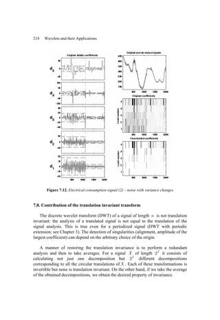
![Signal Denoising and Compression 219
Moreover, these transforms are easy to obtain; it suffices to reuse the DWT
scheme and to remove the decimation phase (for more details see Chapter 3).
The main applications of this transformation are analysis [NAS 95] and,
especially, denoising. The idea of translation invariant denoising, introduced by
Coifman and Donoho [COI 95], consists of carrying out thresholding on each basis
and taking the average of the obtained denoised signals. There are two competing
effects present: a better detection of singularities due to taking into account all the
shifts in the analysis and an effect of more intense smoothing due to the averaging of
the denoised signals on each basis. A good compromise consists of using quite
irregular wavelets with a small support and applying hard thresholding. This strategy
can improve the restitution of the edges and it is also used for denoising images.
Figure 7.13. Translation invariant transform: soft thresholding
Signal (S) and denoised signal (DS) Denoised signal (DS)
Residuals = S – DS
Non-decimated approximation coefficients
Non-decimated approximation coefficients
Non-decimated detail coefficients Non-decimated detail coefficients](https://image.slidesharecdn.com/03-misiti-waveletsandtheirapplications-220602130041-0d67589d/85/03-Misiti_-_Wavelets_and_Their_Applications-pdf-241-320.jpg)


![222 Wavelets and their Applications
The function h can be represented on the wavelet basis constructed using the
functions ϕ and ψ in the following way:
, , , ,
J J
j
J k J k j k j k J
k j k j
h a d A D
ϕ ψ
=−∞ =−∞
= + = +
∑ ∑ ∑ ∑ [7.8]
To estimate h it suffices to estimate the coefficients ,
J k
a and ,
j k
d . By
definition of the coefficients, we have:
( ) ( )
, ,
J k J k
a x h x dx
ϕ
= ∫
As h is a probability density function, ,
J k
a has a particularly useful
interpretation: ( ) ( ) ( )
( )
, , i
J k J k
x h x dx E X
ϕ ϕ
=
∫ is the expectation of the
random variable , ( )
i
J k X
ϕ . Such an expectation is estimated quite simply by the
empirical mean:
( )
, ,
1
1
ˆ
n
i
J k J k
i
a X
n
ϕ
=
= ∑
[7.9]
In the same way we have ( ) ( ) ( )
( )
, , , i
j k j k j k
d x h x dx E X
ψ ψ
= =
∫
estimated by:
( )
, ,
1
1
ˆ
n
i
j k j k
i
d X
n
ψ
=
= ∑
[7.10]
Using the expression of h given by [7.8] and replacing the coefficients by their
estimates given by [7.9] and [7.10], and then by thresholding the estimated detail
coefficients we obtain an estimator h of the form:
{ }
,
0
, , , ˆ ,
ˆ
ˆ 1
I
j k
J
J k j k j k j k
d t
k j J j k
h a d
ϕ ψ
>
= −
= +
∑ ∑ ∑
[7.11]](https://image.slidesharecdn.com/03-misiti-waveletsandtheirapplications-220602130041-0d67589d/85/03-Misiti_-_Wavelets_and_Their_Applications-pdf-244-320.jpg)


![Signal Denoising and Compression 225
We obtain approximations of these estimates by the wavelet coefficients of the
sequence b
Y :
( ) ( )
( )
, ,
1
1
ˆ
m
b b
J k J k
r
a Y r X r
n
ϕ
=
≈ ∑ and ( ) ( )
( )
, ,
1
1
ˆ
m
b b
j k j k
r
d Y r X r
n
ψ
=
≈ ∑
which in this situation also allows us to use the DWT.
Of course, the quality of the obtained estimators is not completely controlled
since it results from the estimation by wavelets, but applied to data transformed by a
kind of preliminary estimate (see [HAR 98] pp. 134 and 183).
7.10. Principle of compression by wavelets
7.10.1. The problem
The problem of compression is often reduced to images, whose applications are
particularly interesting (see Chapter 8). For example, wavelets are used in the new
image compression standard JPEG 2000 [JPE 00].
Nonetheless, the compression of one-dimensional signals is also relevant. Thus,
the legal obligation for certain public service operators to preserve their customers’
consumption curves over long periods necessarily implies their compression.
Similarly, it is crucial to compress audio signals for fast transmissions via the
international network.
Wavelets, with other techniques, contribute to provide effective solutions to this
problem. Of course, the complete compression process includes phases of
quantization, coding and decoding in addition to wavelet processing itself. Should
we concentrate on this, the objective then consists of obtaining the sparse
representation of the signal being compressed. Here we tackle the problem of
compression by wavelets only from this viewpoint.
7.10.2. The basic algorithm
The basic algorithm is very similar to that of denoising and proceeds in three
steps:
− decomposition;](https://image.slidesharecdn.com/03-misiti-waveletsandtheirapplications-220602130041-0d67589d/85/03-Misiti_-_Wavelets_and_Their_Applications-pdf-247-320.jpg)


![228 Wavelets and their Applications
With others wavelets the compressibility curve primarily has the same aspect.
For example, in Figure 7.17, we have represented the curves of compressibility of
the signal and the decompositions by wavelets db1 and sym6 with a logarithmic
scale for the number of coefficients. The more vanishing moments the wavelet has,
the “better” the capacity of compression of the basis.
Figure 7.17. Compressibility curves for the signal, and wavelets db1 and sym6
7.11.2. Selection of coefficients
Other strategies can be used in this context, when the norm chosen to measure
compression quality is not the
2
i norm used above. This can be irrelevant for
perceptual reasons.
In [BIR 97], Birgé and Massart propose a strategy enabling greater flexibility.
They establish a result of the optimal speed convergence for functions f belonging
to Besov spaces. This strategy results in selecting large coefficients at each level.
More precisely, the approximation coefficients at the level J are kept and for each
finer level j J
≤ , only the j
n largest detail coefficients, by absolute value, are
kept. The numbers j
n grow with j as ( )
/ 1
M J j α
+ − where M is a positive
constant and 1
α > is a parameter. The method thus consists of preserving a rough
approximation and selecting few coefficients for the levels of fine details, which
contain high frequency signal fluctuations and more and more coefficients so for the
coarsest levels.
db1
signal
sym6
Percentage
of
energy
captured
Number of preserved coefficients](https://image.slidesharecdn.com/03-misiti-waveletsandtheirapplications-220602130041-0d67589d/85/03-Misiti_-_Wavelets_and_Their_Applications-pdf-250-320.jpg)

![230 Wavelets and their Applications
Figure 7.18. Compression (global thresholding)
The resemblance of the results produced by denoising and compression is
obvious. This is not surprising; it is natural that a good method of compression with
loss leads to eliminate the noise. Indeed, if we compress a noisy signal of the type
defined by [7.1] by preserving the largest coefficients, we will denoise it, at least
partially, since noise coefficients are generally all “small”; this is what occurs in this
example. The difference is that the threshold chosen for compression comes from
external constraint: frequency bandwidth, available memory, prescribed
compression ratios. This is why denoising is not perfect here and fluctuations absent
from the original signal f appear in the compressed signal. On the contrary, in the
case of denoising the technique selects the threshold automatically by estimating the
noise level using the information provided by the model.
7.12.2. A comparison of the two compression strategies
The two strategies described above often yield similar results for reasonable
choices of the parameters. Let us examine, for example, (see the graph on the right](https://image.slidesharecdn.com/03-misiti-waveletsandtheirapplications-220602130041-0d67589d/85/03-Misiti_-_Wavelets_and_Their_Applications-pdf-252-320.jpg)


![234 Wavelets and their Applications
The percentage of zeros obtained is 78.71%. Let us then apply the threshold
leading as previously to 90% of energy preserved in the wavelet packet
decomposition of the signal. The percentage of zeros obtained is now shifted to
88.77%, that is a gain of 10%.
7.14. Bibliographical comments
Let us conclude this chapter with some historical and bibliographical
observations (see Chapter 12 of [MEY 93]). The first papers appeared at the
beginning of the 1990s and powerful ideas emerged very early, for example, in the
work of Donoho, Johnstone, Kerkyacharian, Picard, Doukhan and Antoniadis for
denoising and the work of Coifman, Cohen and De Vore for compression. These
ideas were then developed by many authors. In order to grasp the extent of the
stimulation exerted by these ideas in the statistics and signal community, see [ANT
95].
We find typical results in the rather numerous books dedicated, especially since
1998, to the question of the use of wavelets in statistics. Ogden [OGD 97] offers a
basic presentation thereof. The books by Vidakovic [VID 99] and Percival and
Walden [PER 00] constitute at present the two most complete references in the field.
In the extremely rich book by Mallat [MAL 98], two chapters tackle these questions
from a point of view of signal processing. Several points of our book take this point
of view as a starting point. For a more technical vision see Härdle et al. [HAR 98].
Moreover, see the papers on synthesis by Antoniadis [ANT 97], Antoniadis et al.
[ANT 01] and Abramovic et al. [ABRA 00].](https://image.slidesharecdn.com/03-misiti-waveletsandtheirapplications-220602130041-0d67589d/85/03-Misiti_-_Wavelets_and_Their_Applications-pdf-256-320.jpg)
![Chapter 8
Image Processing with Wavelets
8.1. Introduction
The applications of wavelets in image processing are often synonymous with
compression. Today, the need for storing large quantities of information and for fast
transmission through international communication networks are key issues. This is
why two examples of wavelet used in this field have had a particularly pronounced
impact:
– for fingerprint storage, the FBI finally chose an algorithm containing wavelets
[BRI 95];
– more recently, the compression standard JPEG 2000 [JPE 00] has also been
built around algorithms containing wavelets.
These successes had a resounding echo and contributed to the popularization of
wavelets. For this reason, the last part of this chapter is devoted to what remains the
main 2D-wavelet application: compression.
Before focusing on this point this chapter gives a rapid presentation of the
theoretical framework and considers two of the more marginal but still efficient 2D-
wavelet applications. We introduce the concepts of decomposition, approximation
and detail for an image. They then play a crucial role in:
– the edge detection. In this part we illustrate the capacity of wavelets to locally
analyze the fluctuations of image grayscale levels. The processed examples show
that, almost without processing, the analysis of images by wavelets makes it possible
to extract a new image, from which we can isolate the edges;](https://image.slidesharecdn.com/03-misiti-waveletsandtheirapplications-220602130041-0d67589d/85/03-Misiti_-_Wavelets_and_Their_Applications-pdf-257-320.jpg)
![236 Wavelets and their Applications
– the fusion of images1. Here we crucially use the local character of wavelet
coefficients in order to mix two decompositions stemming from different images.
We first present the problem and the technique used with a simple example. The
second processing, which is more realistic, fuses two fuzzy images, while the last,
less serious processing, amalgamates a mask of the Japanese Nô theater with the
bronze bust of a Roman emperor.
We then use two examples to tackle the techniques of wavelet image denoising,
which prove to be powerful and easy to use. The problem and the procedure are
presented in an example of an artificially noisy image before considering a real
noisy image.
Finally, in the last section we present the principles of compression by wavelets
and then concentrate on aspects specifically related to wavelets before tackling the
complete compression chain with a particular interest in quantization and coding.
This point plays a very important part and has a place in this book for the following
reason. In the preceding version of the JPEG standard (1992), the discrete cosine
transform (DCT) was employed to transform images before coding. The first tests
concerning the use of wavelets in compression, although promising, did not yield
results clearly superior to those of the DCT. The creation and implementation of the
coding algorithm EZW (embedded zerotree wavelet encoding; see [SHA 93]) led to
the development of the JPEG 2000 standard. This algorithm fundamentally exploits
the arborescent nature of the multi-resolution analyses; it is presented at the end of
this chapter and in an appendix at the end of the book.
8.2. Wavelets for the image
Multi-resolution analyses of ( )
2
L were defined in Chapter 2 as a family of
decreasing subspaces having various properties related to approximation, dilation
and translation. Similarly, we can introduce multi-resolution analyses of ( )
2 2
L
(see [DAU 92] Chapter 10, p. 313-315 and [MAD 92]). However, 2D multi-
resolution analyses usually come from constructions using tensor products.
Hereafter we will restrict ourselves to this case.
Starting with a 1D multi-resolution analysis we note the associated
approximation and detail spaces as 1D
j
V and 1D
j
W . For every level j the
approximation space of the 2D multi-resolution analysis is obtained as a sum of four
1D tensor products:
1 Our presentation is based upon the ideas used by P.M. Zeeuw in [ZEE 98].](https://image.slidesharecdn.com/03-misiti-waveletsandtheirapplications-220602130041-0d67589d/85/03-Misiti_-_Wavelets_and_Their_Applications-pdf-258-320.jpg)
![Image Processing with Wavelets 237
( ) ( ) ( ) ( )
2 1 1 1 1 1 1 1 1
1
D D D D D D D D D
j j j j j j j j
j
V V V V W W V W W
− = ⊗ ⊕ ⊗ ⊕ ⊗ ⊕ ⊗
This relation is also written:
2 2 2 2 2
1
D D D D D
j j j j
j h v d
V V W W W
−
⎡ ⎤ ⎡ ⎤ ⎡ ⎤
= ⊕ ⊕ ⊕
⎢ ⎥ ⎢ ⎥ ⎢ ⎥
⎣ ⎦ ⎣ ⎦ ⎣ ⎦
Indeed, 2 1 1
1 1 1
D D D
j j j
V V V
− − −
= ⊗ with 1 1 1
1
D D D
j j
j
V V W
− = ⊕ , which makes it
possible to obtain the first expression for 2
1
D
J
V − .
Whatever the method of 2D construction, whether using tensor products or not,
we have a scaling function, as in 1D, and three wavelets instead of one. In the
particular case of tensor construction, if ϕ and ψ indicate respectively the scaling
function and the 1D wavelet, we have:
– the scaling function: ( ) ( ) ( )
2 ,
D x y x y
ϕ ϕ ϕ
= ;
– three wavelets:
( ) ( ) ( )
2
1 ,
D x y x y
ψ ϕ ψ
= , ( ) ( ) ( )
2
2 ,
D x y x y
ψ ψ ϕ
= , ( ) ( ) ( )
2
3 ,
D x y x y
ψ ψ ψ
=
The algorithms of decomposition and reconstruction of the 2D-DWT, with
preceding tensor construction, are described in Chapter 3.
8.2.1. 2D wavelet decomposition
As in 1D, two types of objects are handled in 2D:
– approximation or detail coefficients corresponding to coordinates in the bases
of spaces 2D
j
V and 2D
j
W ;
– reconstructed approximations and details corresponding to projections on
spaces 2D
j
V and 2D
j
W .
Here we are dealing with monochromatic images, i.e. in grayscale. An integer is
associated with each pixel of the image, which is an index in an ordered table of
“colors”. We speak then of indexed images. Within this framework, an image is then
a matrix of integers. There are, of course, true color images, often associated with
three matrices, for example the RGB coding. We will not cover here the processing
of such images (for additional information see [SKO 01]).](https://image.slidesharecdn.com/03-misiti-waveletsandtheirapplications-220602130041-0d67589d/85/03-Misiti_-_Wavelets_and_Their_Applications-pdf-259-320.jpg)


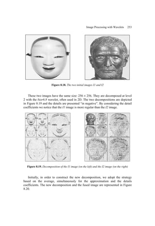


![Image Processing with Wavelets 257
8.5.1. An artificially noisy image
Figure 8.25 presents on the left the original image noted f and on the right the
noisy image noted Z .
Figure 8.25. Original image (on the left), noisy image (on the right)
As in the 1D case we suppose that the image Z is the original image f
corrupted by homogenous additive noise. That is, we consider a model of the type:
,
( , ) ( , ) i j
Z i j f i j ε
= + [8.1]
where Z is the image to be denoised, ε is a white noise with a covariance matrix
2
I
σ and f is the image being restored.
The process of denoising by wavelets consists of three phases:
– wavelet decomposition at the J level of the image to be denoised;
– thresholding, in three directions, of the detail coefficients with smaller absolute
value than a threshold dependent on σ ;
– reconstruction of the denoised image, starting from the approximation
coefficients of level J (unchanged) and of the modified detail coefficients.
We carry out the wavelet decomposition of the noisy image by the Haar wavelet,
at level 4, and obtain the results presented in Figure 8.26.](https://image.slidesharecdn.com/03-misiti-waveletsandtheirapplications-220602130041-0d67589d/85/03-Misiti_-_Wavelets_and_Their_Applications-pdf-279-320.jpg)
![258 Wavelets and their Applications
Figure 8.26. Noisy image (on the left), level 4 decomposition
(in the middle) and level 4 approximation (on the right)
The principle of denoising is simple. We start with a coarse version of the image,
here the level 4 approximation and then we select detail coefficients to construct the
necessary touching up in order to improve the result.
We will present three successive tests, without specifying the choice of
thresholds but focusing on the results (see [MIS 00]).
Let us begin by thresholding the Haar decomposition coefficients seen in Figure
8.26. The threshold is obtained by estimating σ and applying a penalization
strategy.
Original image Denoised image
Figure 8.27. Noisy image (on the left) and image denoised by Haar (on the right)](https://image.slidesharecdn.com/03-misiti-waveletsandtheirapplications-220602130041-0d67589d/85/03-Misiti_-_Wavelets_and_Their_Applications-pdf-280-320.jpg)

![260 Wavelets and their Applications
The result is very satisfactory from the point of view of noise. On the other hand,
we note a loss of definition of the edges and the denoised image is fuzzy.
Figure 8.29. Noisy image (on the left) and image denoised by the SWT (on the right)
After this example in which we added “a good” noise to a good quality image,
let us move on to a noisy image obtained via an uncontrolled process.
8.5.2. A real image
The image to be denoised is presented in Figure 8.30. It is a real image coming
from the digitalization of an ID photo. It is of a rather bad quality, as can be seen
from the hair, for example. An additional noise seems to have been superimposed on
the original image and, moreover, white spots are deteriorating the texture of the
face.
We try to improve the image by applying denoising methods similar to those
seen previously. Let us consider again the model [8.1]:
,
( , ) ( , ) i j
Z i j f i j ε
= +
where f , the image to be restored, is in this case the initial ID photograph.
Let us first apply the denoising method by SWT using the wavelet sym6 and
decomposing at level 3. The result is shown in Figure 8.31.](https://image.slidesharecdn.com/03-misiti-waveletsandtheirapplications-220602130041-0d67589d/85/03-Misiti_-_Wavelets_and_Their_Applications-pdf-282-320.jpg)


![270 Wavelets and their Applications
coding does not involve any loss of information. Now let us detail each of these two
operations.
8.6.3.1. The quantization
The coefficients obtained by applying the DWT and thresholding to an image are
generally real numbers. Sometimes they are integers, but their variation domain is
large. The quantization phase consists of approximating the set of values of the
coefficients by a finite set of numbers and, in general, implies a loss of information.
Let E be a set, P a finite partition of E and F a set containing one and only one
element of each class of the partition P. The quantizer q associated with ( )
, ,
E P F
is the application for which x̂ F
∈ is the image of x E
∈ . If K
E ⊂ we refer to
a vector quantizer and if E ⊂ , we refer to a scalar quantizer.
Let us give a simple example of a quantizer:
[ ]
0,1
E = ,
6
1 1 1 2 5 5
6 6 3 3 6 6
1
0, , , ,1 k
k
P I
=
⎡ ⎡ ⎡ ⎡ ⎡ ⎡ ⎡ ⎤
= ∪ ∪ ∪ ∪ =
⎣ ⎣ ⎣ ⎣ ⎣ ⎣ ⎣ ⎦ ∪ and
{ }
5
1 2 3 4 6
, , , , ,
F e e e e e e
= with k k
e I
∈
How can we choose class representatives, i.e. i
e ? The error of quantization for
the set { } 1
N
n n
X x =
= of given elements of E is measured by a distance between
X and ( ) { } 1
ˆ ˆ N
n n
X q X x =
= = , the set of values obtained by quantization. In
general, we take the average quadratic error:
( )
2 2
1
1
ˆ ˆ
,
N
n n
n
d X X x x
N =
= −
∑
If a probability distribution E exists, the quantization error is measured by the
expectation D of the mean square error.
0 1
2
e 3
e 4
e 5
e 6
e
1
e](https://image.slidesharecdn.com/03-misiti-waveletsandtheirapplications-220602130041-0d67589d/85/03-Misiti_-_Wavelets_and_Their_Applications-pdf-292-320.jpg)
![Image Processing with Wavelets 271
Let us continue the preceding example and provide [ ]
0,1
E = with the uniform
probability. The best choice for the set F, minimizing the distortion D, is obtained
by taking the middle of each partition segment for i
e :
{ }
7
1 3 5 9 11
12 12 12 12 12 12
, , , , ,
F =
We will now show the effects of quantization on the visualization of the
fingerprint. This indexed image corresponds to a matrix of integers ranging between
0 and 255. Through quantization we can decrease the number of usable colors, here
256. Figure 8.42 illustrates the passing from 256 to 16 colors. We see at the top left,
the original image, at the top right, the histogram of values, then at the bottom right,
the histogram of quantized values and at the bottom left, the reconstructed image.
The classes are delimited by dotted lines and their center is illustrated by a dot. The
effective interval of values is [ ]
19,152 and it is quantized into eight classes.
Figure 8.42. Example of quantization of the original image: a fingerprint
0 1
2
e 3
e 4
e 5
e 6
e
1
e](https://image.slidesharecdn.com/03-misiti-waveletsandtheirapplications-220602130041-0d67589d/85/03-Misiti_-_Wavelets_and_Their_Applications-pdf-293-320.jpg)

![Image Processing with Wavelets 273
8.6.3.2. EZW coding
Once transformation and quantization have been performed we have a finite
sequence X̂ of elements belonging to a finite set of symbols S . The objective of
coding is to represent in the best possible way, for example by a sequence of 0 and
1, the sequence X̂ according to predefined objectives.
We now have to code X̂ in the most efficient way possible. In general, this
means the most economic way possible, i.e. by minimizing the quantity of
information used to describe this set. This is the main objective of data compression.
Thus presented this problem does not have a direct connection with wavelets; it is a
common problem and studied widely in information theory. There are many
manners of building a code, let us outline some of them.
The first idea is to code each symbol of S using a binary fixed length word
(fixed length code). Thus, we obtain a sequence of 0 and 1 coding the sequenceX̂ .
From the point of view of compression this method offers practically no interest.
The second idea consists of exploiting the fact that X̂ contains a large quantity
of zero values. We can then code the most frequent symbols with shorter sequences
(variable length code). This reduces the quantity of information necessary to
represent X̂ . We can also code only the non-zero values of X̂ , but their positions
should then also be coded. This method, allied to Huffman type coding or semi-
arithmetic or arithmetic codings [HUF 52], [AHO 87], [MAL 98], [WIT 87], [HOW
92], leads to satisfactory compression performances, comparable with those of JPEG
92.
The third idea, which is critical for the use of wavelets in image compression, is
to fundamentally exploit the tree structure of the wavelet decomposition. Certain
codes developed from 1993 to 2000 use this idea, in particular, the EZW coding
algorithm introduced by Shapiro [SHA 93], which we will now consider.
The EZW algorithm is based on progressive coding of data. On the one hand,
this makes it possible to obtain during decoding an image whose precision, i.e.
resolution, increases gradually. In addition, it is possible to obtain a sequence of
compression ratios based on the length of the retained code. This compression
usually involves a loss of information, but the algorithm also enables compression
without loss.
Generally, real images have a low frequency spectrum. Wavelet decomposition
transforms them into a set of large (on average) approximation coefficients and
detail coefficients that are on average always growing with the scale.](https://image.slidesharecdn.com/03-misiti-waveletsandtheirapplications-220602130041-0d67589d/85/03-Misiti_-_Wavelets_and_Their_Applications-pdf-295-320.jpg)


![276 Wavelets and their Applications
Figure 8.46. EZW algorithm: at the top, results after 1, 2, 3, 4 and 5 iterations; in the
middle, results after 6, 7, 8, 9 and 10 iterations; at the bottom on the left, results
after 11, 12 and 13 iterations, and at the bottom on the right the original image
8.6.3.3. Comments on the JPEG 2000 standard
In addition to operations linked to wavelets (DWT and IDWT) and the aspects
associated with coding and quantization, the JPEG 2000 method comprises many
technical subtleties. It is the effectiveness of the system on the whole which led to
JPEG 2000 becoming the standard for image compression (see [SKO 01] and [JPE
00]); here we will only provide some indications.
The JPEG 2000 system was constructed to satisfy three major objectives. First of
all, to offer a certain universality: for a broad family of color images to achieve
better performances than existing standards for strong compression ratios, without
degrading them for lower ratios. Then, to enable a progressive transmission of
compressed images with increasing quality until a lossless compression is achieved
and to make it possible to define specific areas that have to be coded with greater
precision. Lastly, to ensure good data security and robustness with respect to errors
during transmission.](https://image.slidesharecdn.com/03-misiti-waveletsandtheirapplications-220602130041-0d67589d/85/03-Misiti_-_Wavelets_and_Their_Applications-pdf-298-320.jpg)


![Chapter 9
An Overview of Applications
9.1. Introduction
9.1.1. Why does it work?
As this chapter shows, wavelets are used in a large number of fields. Let us just
mention geophysics, astrophysics, quality control, biology and aural signals in
medicine, imagery in all its aspects and medical imagery in particular, compressed
representation of fingerprints or photographs, satellite imagery, coding of video
signals, modeling of traffic in communication networks like the Internet and analysis
of atmospheric or wind tunnel turbulence. Even after years of work we remain
surprised by the variety of domains concerned and the problems dealt with.
A question arises from the start: how is it possible that the same tool works for
so many applications? Of course, it is impossible to find a single really satisfactory
answer, but several reasons appear plausible. In his book of historical presentation of
wavelets, Hubbard (see [HUB 95] p. 139-173) proposes several clues on very
diverse levels:
− first of all, the wavelets method is new in signal processing. It brings technical
innovations and makes it possible to look at traditional information through original
easily accessible tools. A new dictionary of shapes is created, connecting signal
characteristics to those of wavelet transforms, enabling us to infer properties of the
signals based on coefficient structures. There are, for example, visible cones in
continuous decomposition, which indicate a serious signal irregularity. It is also
known that zero coefficients in a discrete decomposition indicate that the signal is](https://image.slidesharecdn.com/03-misiti-waveletsandtheirapplications-220602130041-0d67589d/85/03-Misiti_-_Wavelets_and_Their_Applications-pdf-301-320.jpg)


![An Overview of Applications 283
9.1.3. Two problems in which the wavelets are competitive
Denoising and compression are two problems solved well by wavelets and are,
nonetheless, still subject to development. The techniques are detailed in Chapters 7
and 8. We only summarize some useful ideas in the application files, where they
have not yet been included.
Denoising
The general spirit of modeling distinguishes the useful signal from the noise.
Noise reduction, which consists of, according to the beautiful expression of V.
Wickerhauser quoted in [HUB 95], “cut the weeds and spare the daisies”, includes:
− suppression of noise to locate great, often slow, evolutions associated with the
trend or smooth zones;
− search and modeling of non-smooth parts varying quickly but stable enough,
characterized by flat spectra whose most usual representative is white noise, or by
textures, zones exhibiting a repeating pattern;
− suppression of the irrelevant part to preserve the interpretable part.
We come across denoising in several of the applications indexed in this chapter.
Compression
Compression compacts information to preserve or transmit it. To some extent, it
bears a greater resemblance to denoising, with which it shares an end of the
technical processing chain. However, apart from noise reduction, it optimizes a
criterion which is a direct function of the scarcity of the coefficients preserved – in
the sense that it is a question of restoring the original object in the most accurate
manner possible with some information given a priori.
9.1.4. Presentation of applications
In order to conclude this introduction in the rows of Table 9.3 we find the
applications detailed in the rest of this chapter and, in the columns, the topics or the
fields with respect to which they are introduced.](https://image.slidesharecdn.com/03-misiti-waveletsandtheirapplications-220602130041-0d67589d/85/03-Misiti_-_Wavelets_and_Their_Applications-pdf-305-320.jpg)

![An Overview of Applications 285
9.2. Wind gusts
Objective
In [LIU 94] the objective is to characterize ocean winds during their formation
phase, their growth and the period of full development.
Data
Measurements of wind and wave heights were made during the large storm on
October 26, 1990 at sea (Atlantic Ocean), on the basis of 10 recordings a second,
producing 100 sets of 1,024 measurement points and covering the total duration of
the storm. The intensities of winds range between calm and strong winds of 18 m/s
(64.8 km/h). The waves reach 7 meters in height.
Technique
The spectrum, cospectrum, coherence and quadrature are usually defined and
studied by spectral analyses. These concepts adapt to the wavelets framework by
replacing the base of the complex exponentials intervening in Fourier with wavelets
,
a b
ψ . The energy of the decomposed signal is then analyzed according to time and
scale. For one-dimensional signals the analysis is traditional. For signals with two or
more dimensions processed simultaneously, the study becomes multivariate and then
more specific.
If X and Y are time-series and X
C and Y
C are the corresponding continuous
decompositions, then for a wavelet we define:
− wavelet spectrum:
( ) ( )
2
, , )
X X
W a b C a b
=
− wavelet cross spectrum:
( ) ( ) ( )
, , ,
XY X Y
W a b C a b C a b
=
− coherence:
( , )
( , )
( , ) ( , )
XY
X Y
W a b
a b
W a b W a b
=
Coher](https://image.slidesharecdn.com/03-misiti-waveletsandtheirapplications-220602130041-0d67589d/85/03-Misiti_-_Wavelets_and_Their_Applications-pdf-307-320.jpg)

![An Overview of Applications 287
Figure 9.1. (Extracted from [LIU 94] p. 159): wind speeds are represented in the upper part
of the figure. The lower part shows the wavelet spectrum of the signal using the Morlet
wavelet. Time is measured along the x-axis and frequencies are located along the y-axis.
The energy is constant for each contour line. These lines delimit the time
and frequency zones of strongly energetic wind
Role of the wavelets
As usual, wavelets analyze the local distribution of the energy of a scalar signal.
They also compare time shifts and phase shifts, which appear in a couple of signals.
They supplement the possibilities offered by the cospectra of the Fourier analysis.
9.3. Detection of seismic jolts
Objective
In [ANA 97] the issue is to automatically identify various components, usually
called P and S, of a seismic signal, short and non-stationary, using wavelets as a tool
of pattern recognition.
The seismogram records motion in three directions: two in the horizontal and
one vertical. Usually, the location is based on several ground detectors. We may,](https://image.slidesharecdn.com/03-misiti-waveletsandtheirapplications-220602130041-0d67589d/85/03-Misiti_-_Wavelets_and_Their_Applications-pdf-309-320.jpg)


![290 Wavelets and their Applications
Figure 9.3. (Extracted from [ANA 97]): two shapes of seismic signals and zooms around the
event. We can compare the shapes of the start of the signals and the shapes
of the wavelets in Figure 9.2 and note that they correspond well
9.4. Bathymetric study of the marine floor
Objective
In [LIT 94] the issue is to chart marine floor areas in order to locate shapes and,
in particular, to locate the strong escarpment declivities. The zone covered is in the
North Atlantic and shows a central valley oriented S/E-N/W, zone of the tectonic
plates separation, framed by escarpments. It measures 100 km × 70 km. The depths
vary between 1,800 m and 4,000 m.
Data
An “echo sounder” mounted on a boat traversing the zone to be covered collects
the signal. The typical image has as a size of 755 points along the longitude
direction by 495 along the latitude direction.
Technique
It is a technique of image improvement and pattern detection of shapes by using
a wavelet based on B-splines tensored with a filter. The function is rotated in the
plane so that its principal direction will be that of the required edges. The derivative
of the cubic B-spline provides another function, which locates the transitions
between valleys and escarpments.](https://image.slidesharecdn.com/03-misiti-waveletsandtheirapplications-220602130041-0d67589d/85/03-Misiti_-_Wavelets_and_Their_Applications-pdf-312-320.jpg)
![An Overview of Applications 291
Results
The required shape is a long, rectilinear, narrow edge whose dominant
orientation is parallel to the axis of the expansion of the earth’s crust. To locate this
shape, the wavelet acts mainly as an edge detector. Figure 9.4 shows the results. The
required lines are parallel to the central valley. They are difficult to locate on the
basic decompositions and are discovered much better through the visualization of
local minima and maxima (by traversing the image from the East to the West).
Role of the wavelets
“The wavelets decomposition of bathymetric data reveals structures and patterns
which are easily overlooked in the raw data”. The wavelet produces: “a qualitative
image enhancement and a qualitative fault scarp identifier”. “Wavelet analysis offers
a useful method for decomposing the texture of the seafloor to help understand
processes which occur at many different scales” (quotations extracted from [LIT
94], p.167 for the first and p. 180 for the two following ones).
Figure 9.4. (Extracted from [LIT 94]): detection of edges on the bathymetric
image of the marine floor using a wavelet based on B-splines
9.5. Turbulence analysis
Objective
The study of Papanicolaou and Solna [PAP 01] deals with the famous
Kolmogorov turbulence law, which links energy to scale. It provides a](https://image.slidesharecdn.com/03-misiti-waveletsandtheirapplications-220602130041-0d67589d/85/03-Misiti_-_Wavelets_and_Their_Applications-pdf-313-320.jpg)
![292 Wavelets and their Applications
phenomenological description of the velocity field in the atmosphere and is
expressed by a power law. The average square of the increments of the velocity x
V ,
for a large range of scales, is modeled by
( ) ( )
( ) 2/3
2 2
0 0
x x v
E V x u V x C u
⎡ ⎤
+ − =
⎢ ⎥
⎣ ⎦
.
The important thing in this formula is its power form and the order of magnitude
of the coefficient (here 2
3 ).
The two basic ingredients of this type of study are:
− on the one hand, the model of the process called fractional Brownian motion
and noted H
MBF (which is the French abbreviation) which depends on a parameter
H (or one of its extensions which allows the variation of H );
− on the other hand, the wavelet spectrum, which generalizes the usual spectrum
based on the Fourier transform.
The wavelets harmoniously introduce the decompositions according to the scales
involved in various estimation techniques.
Let us say a word on the fractional Brownian motion H
MBF . It is a continuous-
time process, which resembles a usual Brownian motion whose derivative is a white
noise. It is Gaussian, self-similar in distribution and the variance of the increments
depends on H in the following way:
( ) ( )
( ) 2 2H
H H
Var MBF t MBF s t s
σ
− = − .
The extension of H
MBF to the ( )
H t
MBF or ( )
H
MBF λ , making it possible to
make H depend on time or frequency, is important since situations compatible with
models with a constant parameter seem rare. These new objects are used, for
example, in the modeling of vertical turbulence. Additional information can be
found, for example, in [BOS 00] and [DOU 03].
Data
The data comes from a lidar emitting a laser beam, delivering measurements
from which atmospheric temperatures at various altitudes are deduced. The
recordings are long and include n = 4,200,000 vertically spaced points of 2 cm. They
cover a vertical more than 80 km long.](https://image.slidesharecdn.com/03-misiti-waveletsandtheirapplications-220602130041-0d67589d/85/03-Misiti_-_Wavelets_and_Their_Applications-pdf-314-320.jpg)
![An Overview of Applications 293
Technique
The very first methods of decompositions of DWT type using around 20 dyadic
scales show that any modeling, which would provide a power law, should allow the
parameter representing power to vary with altitude. The model is then local.
The work consists of finding a partition of the vertical line (altitude) and
calculating the corresponding estimates of H . The technique is as follows:
− choice of the bands of values where the parameter can be regarded as constant;
− estimation of the values of H , parameter which varies with the segment.
Results
We know that, according to the value ofH , the memory of the process is short
or long. The results locate
1
3
H in the zone of the short memory values,
corresponding to a theoretical spectrum of increments of the shape
5
3
λ
−
in the
neighborhood of the 0 frequency.
An important part of statistical work consists of:
− determining segments in which H can be regarded as constant, segments
which, in order to ensure a precise estimate, must be as large as possible;
− verifying that the estimates do not depend too much on the partitioning. The
vertical is partitioned into segments of 655 m, a value determined following many
tests. Energy analyses make it possible to notice that low altitudes present lower
energy than the high ones [PAP 01].
The statistical technique is based on several ideas, including the one that
connects in one H
MBF the variance of the wavelet coefficients at level j to j
itself. The estimate Ĥ of H is obtained by regressing the logarithm of this variance
over the logarithm of j . The study is a little more complicated and a modeling of
H using a random walk is introduced.
The only wavelet used in this study is the Haar wavelet. The scaling function
ϕ does not appear. In fact, only the multi-resolution aspect is useful, at the expense
of other wavelet properties. The wavelet simultaneously carries out the calculation
of the increments of the measurements and the low frequencies filtering.
Percival and Guttorp [PER 94] study a similar problem concerning vertical
shearing forces in the ocean. The data are collected every 0.1 m, differentiated and
pre-filtered in order to preserve the non-noised evolutions. A reasonable model](https://image.slidesharecdn.com/03-misiti-waveletsandtheirapplications-220602130041-0d67589d/85/03-Misiti_-_Wavelets_and_Their_Applications-pdf-315-320.jpg)
![294 Wavelets and their Applications
postulates the evolution into power law ( )
S α
λ λ
= of energy according to depth,
at least for a rather broad range of scales. The model is estimated by the use of SWT
wavelet decomposition, needed for the calculation of the variance of the wavelet
coefficients for each scale level. This estimator is linked to the Allen variance,
famous in the non-stationary signal processing.
These studies are useful in the modeling of turbulence because they specify the
link between interesting and difficult to model data, the local power law, Brownian
modeling and wavelets.
9.6. Electrocardiogram (ECG): coding and moment of the maximum
Objective
In [ANA 95] the issue is the adequate coding of the wavelet analyses of long
signals. This problem arises for biomedical signals for the purposes of storage and
transmission. The compression ratio must be increased while maintaining the
distortion at an acceptable level in order to allow a clinical examination. The
essential shapes of the cardiac electric signal are the P shapes, the QRS complex and
the T shape (see Table 9.4).
There are classical coding techniques. They are based on “DPCM (scalar and
vector coding), entropy coding, Fourier or Walsh transformations” [ANA 95].
An ECG is a short and quickly variable signal and is, thus, a good candidate for
wavelet analysis. The amplitude, duration and rhythm enable the identification of
the anomalies. The operation of the cardiac muscle is described on the basis of the
elements of Table 9.4.
Characteristics of the wave Activity
P Electric activation of Atria
QRS Electric activation of the ventricles
P-QRS Time Duration of Atria-Ventricle electric conduction
T Repolarization of the ventricles
Table 9.4. The essential shapes of the cardiac electric signal](https://image.slidesharecdn.com/03-misiti-waveletsandtheirapplications-220602130041-0d67589d/85/03-Misiti_-_Wavelets_and_Their_Applications-pdf-316-320.jpg)
![An Overview of Applications 295
Data
100 ECGs are analyzed by three wavelets: the db12, a Vetterli-Herley wavelet
and a biorthogonal wavelet.
Technique
Scalar and vectorial codings are used on different scale bands. The former for
small scales with signals changing quickly; the latter for long and slowly changing
signals. The wavelet decomposition goes up to level 5.
The coding dictionary is built around the sequences 5 5 1
, ,...,
a d d by the
algorithm of average points (k-means) and the average points are the codes. The
number of learning vectors is large and depends on the scale.
Results and advantages of wavelets
The gain is significant compared to the usual methods. The two evaluation
criteria are the bit per sample ratio and a quadratic error of reconstruction. The
Vetterli-Herley wavelet produces the best results.
Supplements to an older work
The study [ANA 94] proposes an estimate of the moment of the maximum of the
wave P using wavelets. We start with many cardiac cycles, which are signals of
length 316 points. We construct a study data set by associating to each cycle 4 new
signals constructed by moving the P wave and the QRS complex at random.
Decomposition uses a quadratic spline wavelet with compact support and
wavelet coefficients of a single scale constitute the data input of the research
procedure for the moment of maximum. A neural network determines the required
moment. We compare the rough data processing with that of the wavelet
coefficients. The qualities are similar, the wavelet analysis is used here as a
preprocessor for the main treatment and saves the quantity of processed information.
From this point of view the wavelet is useful.
9.7. Eating behavior
Objective
Tate [TAT 95] and [TAT 96] studies the influence of the type of fat ingested by
an individual on the fat stored by the body. The basic measurement is a magnetic
resonance spectrum providing information on the chemical composition of fat. The
peaks of the spectrum represent nuclei in various molecular sites, resonating at](https://image.slidesharecdn.com/03-misiti-waveletsandtheirapplications-220602130041-0d67589d/85/03-Misiti_-_Wavelets_and_Their_Applications-pdf-317-320.jpg)
![296 Wavelets and their Applications
slightly different frequencies. The surface located under each peak estimates the
quantity of the substance associated with the peak. In vitro, the peaks are pointed. In
vivo, the identification of the peaks is much more difficult, so much so that it is
desirable to avoid it.
Data
The database is a set of spectra
13C of subcutaneous fat taken from patients’
thighs. The volunteers are either vegans ( 33
n = ), vegetarians ( 8
n = ), or meat
eaters ( 34
n = ). A pre-processing realigns the spectra based on the largest peak;
512 points are preserved and the total energy is normalized to 1.
Technique
Each spectrum is broken up into its wavelet coefficients by the db20, recoded
using the first 64 coefficients. A discriminant factorial analysis classifies the set of
the 75 spectra without it being necessary to measure or to identify the peaks of the
spectra.
Results
A jackknife technique makes it possible to select the best discriminant factorial
components, thereafter used in the discrimination stage. The properties of good and
bad classifications are indexed in Table 9.5.
Good
classification
Bad
classification
Rate of good
classification
Vegetarians excluded 63 4 94%
Vegetarians included 60 15 80%
Table 9.5. Discriminant results obtained using wavelet-based classification
These results improve the previous studies using spectrum peaks’ energies, in
which 20 cases were classified badly when the vegetarians are included and 5 when
they are excluded (see [TAT 96]).
Advantage of wavelets
Although working blind, without information on the signal to be analyzed,
wavelets select information by strongly reducing its quantity. The later statistical
stages are simplified and the quality of classification improved.](https://image.slidesharecdn.com/03-misiti-waveletsandtheirapplications-220602130041-0d67589d/85/03-Misiti_-_Wavelets_and_Their_Applications-pdf-318-320.jpg)
![An Overview of Applications 297
9.8. Fractional wavelets and fMRI
Objective
The purpose of the article [FEI 00] is to discuss the determination, in a rather
broad family, of the wavelet to choose in order to ensure a good analysis of the
fMRI (functional magnetic resonance imaging) data. Optimization is done for
known activation patterns.
Functional imagery highlights the cortical zones of a patient, activated by
external stimulation or during a cognitive or motor task.
Data
The research in the large majority of works is structured by an experimental
design whose factors are the subjects and the working conditions. Let us note
( )
,
A
I x y
τ
and ( )
,
B
I x y
τ
a sequence of images indexed by the time τ for the two
conditions A (activation) and B (rest), and pose:
( ) ( ) ( )
, , ,
D B
A
I x y I x y I x y
τ τ
τ
= −
Prior to any treatment, the data are realigned; a motion correction is enforced and
drifts in time are removed.
Technique
The family of wavelets considered, called fractional splines, generalizes the B-
splines and was introduced by Unser. It is constructed on the basis of power
functions x n α
+
− where ( )
max ,0
x x
+ = and exists in causal and non-causal
symmetrical, biorthogonal or orthogonal shapes. The associated filters do not have a
finite impulse response but are, nevertheless, simple. The design parameter used for
optimization is α .
To detect an activation we calculate the wavelet coefficients W
I
τ
of D
I
τ
. A
statistical test on the coefficients makes it possible to reduce noise and then to
evaluate the significance of activation.
In an fMRI the traditional technique is called SPM (statistical parameter
mapping). It filters the images before the statistical test. The pre-filtering
complicates the situation by making the noises of various pixels of the resulting
image dependent.](https://image.slidesharecdn.com/03-misiti-waveletsandtheirapplications-220602130041-0d67589d/85/03-Misiti_-_Wavelets_and_Their_Applications-pdf-319-320.jpg)
![298 Wavelets and their Applications
Results and role of the wavelets
The zero hypothesis of the statistical activation test concerning the pixel ( )
,
x y
is ( )
( )
, 0
W
E I x y = . The test is based on a Student’s t distribution,
( )
( )
,
,
W x y
I
t
s x y
= , where ( ) ( )
1
1
, ,
n
W W
I x y I x y
n τ
τ=
= ∑ and ( )
,
s x y is the standard
deviation of ( )
( ) 1, ,
,
W n
I x y
τ τ=
. As the test bears on each pixel, the fine-tuning of
the critical value tthreshold is done, as usual, using conservative techniques.
Optimization proves to be important. The selected criteria differ for simulated
and real data. In both cases the gain is large between an optimized choice and a
merely reasonable choice.
The new wavelets are better than the tested Daubechies wavelets. We also find
that:
− causal wavelets are better than symmetrical ones, the former presenting a
better spatial localization;
− biorthogonal and orthogonal wavelets are better than the Daubechies wavelets,
at least when the noises are large;
− the optimal degree α differs from one situation to another. It is close to 1 in
the following expression of the biorthogonal filter of the two scales relation for the
scaling function ( )
1
1
1
2
2
z
H z
α+
−
⎛ ⎞
+ ⎟
⎜ ⎟
= ⎜ ⎟
⎜ ⎟
⎜
⎝ ⎠
. To implement the test it is rare that
the wavelet decomposition requires more than two levels.
Detection is considered to be, on the whole, effective and robust with respect to
the different sizes of the activated zone and to the noise. “Because of its multi-
resolution nature, our method is especially suited for detecting shapes with various
frequency contents, such as mixtures of large and tiny activation zones” [FEI 00].
9.9. Wavelets and biomedical sciences
Objective
We focus here on a very interesting synthesis paper [UNS 96] which, although
published in 1996, still gives a broad, very clear and relevant review of the
applications of wavelets in biomedical sciences.](https://image.slidesharecdn.com/03-misiti-waveletsandtheirapplications-220602130041-0d67589d/85/03-Misiti_-_Wavelets_and_Their_Applications-pdf-320-320.jpg)

![300 Wavelets and their Applications
− the analysis by level of scale provides a technique of detection of shape and,
thus, constitutes a zooming tool (see Chapter 5). Here is the reason: if a signal in an
unknown 0
t point and on an unknown 0
a scale resembles the shape of the wavelet
0
0
t t
a
ψ
⎛ ⎞
− ⎟
⎜ ⎟
⎜ ⎟
⎟
⎜
⎜
⎝ ⎠
, the associated wavelet coefficient is large and makes it possible to
estimate 0
t and 0
a . This property is used to study spikes in the EEG of epileptic
patients as well as in the detection of complex QRS from the ECG;
− the wavelets having zero spectra in the vicinity of the 0 frequency and even
“very” zero (the zero is of an order higher than one) make it possible to make the
colored noises whiter. By filtering the noise by convolution, the wavelet seen as a
filter multiplies the signal spectrum by that of the filter and cancels the energy at
low frequencies. Thus, filtering renders nearly independent the noises with a long
memory whose spectrum ( ) ( )
2 1
H
f λ λ− +
∼ is infinite, with
1
1
2
H
< < in the
vicinity of 0
λ = ;
− wavelets ensure a simultaneous time-scale analysis and compete with time-
frequency analysis tools, which are the short-time Fourier transform, also called the
Gabor transform (see Chapter 2), or the Wigner-Ville analyses.
9.9.1. Analysis of 1D biomedical signals
9.9.1.1. Bioacoustic signals
The analysis of aural signals emitted by the heart, classified into “sounds and
murmurs” constitutes a basic monitoring technique. The wavelets supplement the
usual time-frequency techniques, separating components that are difficult to
dissociate (like “aortic and pulmonary valve components” [UNS 96] p. 630). The
more diffuse sounds are modified by vasodilator drugs and the changes are
appraisable by wavelets, thus enabling the experiments on the classification of
subjects suffering from coronary disease.
9.9.1.2. Electrocardiogram (ECG)
The cardiac signal breaks up into sequences, the most important of which is
called the QRS complex. The location of shape by wavelets makes it possible to
discriminate between normal and abnormal patterns. Wavelets tested on a usual
database prove to have an excellent rate of detection. Although the other methods
could not locate them, the wavelets clearly detect small signals with rather high
frequency appearing in the coronary diseases, infarctions or ventricular arrhythmias.](https://image.slidesharecdn.com/03-misiti-waveletsandtheirapplications-220602130041-0d67589d/85/03-Misiti_-_Wavelets_and_Their_Applications-pdf-322-320.jpg)
![An Overview of Applications 301
9.9.1.3. Electroencephalogram (EEG)
Wavelets have proven reliable in the location of transitory characteristic signals
mixed with normal signals. As the seizure increases, “the transient activity slowly
develops into more nearly regular high amplitude quasi-periodic oscillations” [UNS
96]. Very different depending on the patients, complex signals remain quite
analyzable. Studies for neurosurgery with implanted electrodes developed fast
algorithms for continuous analysis. When the electrodes are on the scalp, the
background electromyogenic noise interferes with the signal. The wavelets have also
been used in the works of discrimination on the functioning of the fetus’s brain.
The action of an external stimulation to the patient is visible on the EEG,
whether this stimulation is acoustic, visual or somatic. The noises are averaged
across a great number of repetitions, typically a few hundred. Stimulation is
locatable after a time of latency. The evaluation of this time, based on the
distribution of the coefficients energy, enables a reliable estimate of the time
evolution of a neurological attack such as cerebral anoxia.
9.9.2. 2D biomedical signal analysis
The most traditional application in biomedical signal analysis is noise reduction.
Another is to increase image contrasts. In mammography, where a very small
change of fabric structure can reveal the presence of a tumor or a micro calcification,
wavelets are effective to detect such events.
9.9.2.1. Nuclear magnetic resonance (NMR)
Subjected to an external magnetic field of controlled frequency, the spins of the
nuclear cores respond and increase their energy. The signal records the emissions
coming from the return of the spins to the realignment position. The recording is
done in a prescribed portion of space made up, for example, by a section. The
measurement of the space density of the resonating spins provides information on
the state of the excited medium.
An integral formula that has to be inversed connects the measured variable to the
space density. Usually the inversion is done in the Fourier base. The wavelets enable
faster calculations and reduce the artifacts ascribable to the movements of the
patients.
In tomography the fMRI uses the multi-resolution aspects of the wavelets. “The
information at different scales is updated at different rates; in particular, low
frequency components can be reconstructed almost instantaneously and used to](https://image.slidesharecdn.com/03-misiti-waveletsandtheirapplications-220602130041-0d67589d/85/03-Misiti_-_Wavelets_and_Their_Applications-pdf-323-320.jpg)
![302 Wavelets and their Applications
estimate the motion of the object” [UNS 96], an estimate which, in turn, contributes
to the determination of the fine structures.
9.9.2.2. fMRI and functional imagery
fMRI is a research tool in neurosciences. It studies “the neural activity of the
brain in vivo” and records, for example, spatial distribution of radiotracers whose
local changes are being followed. It is integrated in an experimental planning whose
factors are the subjects and the conditions.
The images are extremely noisy and variable. A multi-resolution analysis based
on splines ensures the representation of the images and volumes.
In order to distinguish activation from non-activation, the comparison is made
pixel by pixel after control and compensation for the anatomical differences between
subjects and the movements of each subject. Once realigned, the data is submitted to
statistical tests carried out in the wavelet domain, i.e. on the coefficients, thus
avoiding the noise and concentrating on the smoothest parts which are more
meaningful for the image.
The advantages of wavelets over the more traditional methods are as follows:
− wavelets recode information in a small number of large value coefficients;
− the signal-to-noise ratio of these coefficients is good if we find ourselves in the
rather common situation where the noise is about the same everywhere in the
measurement space. A good signal-to-noise ratio ensures a good detection rate;
− finally, wavelets often have the capacity to decrease space dependences
enabling the use of simple statistical tests.
9.10. Statistical process control
Objective
The statistical process control (SPC) is a set of methods, integrated into quality
control, enabling the development of procedures for designing, controlling and
monitoring industrial and manufacturing processes. They are based on the modeling
of normal operation, called controlled (or under control) operation, and on the
definition of situations of abnormal operation indicated by the term out of control. A
monitoring statistic is calculated and controlled regularly during successive
samplings. As long as it remains in the controlled zone, the following sampling is
carried out. As soon as it enters the out of control zone, production is stopped and
the search for causes which provoked the dysfunction is initiated. The monitoring](https://image.slidesharecdn.com/03-misiti-waveletsandtheirapplications-220602130041-0d67589d/85/03-Misiti_-_Wavelets_and_Their_Applications-pdf-324-320.jpg)
![An Overview of Applications 303
statistics most usually employed are Student’s t or its multivariate version called
Hotelling’s 2
T . Successive values are visualized on a chart exhibiting the index of
the batch along the x-axis and the value of t or of 2
T along the y-axis.
When several simultaneous measurements are available, the problem is
multivariate nature and the investigation into the causes becomes crucial and
difficult. Despite their apparent complexity, the majority of multidimensional
recordings depend only on a small number of dimensions: often two, sometimes
three, seldom more, although the theoretical approach does not limit this number.
The principal component analysis makes it possible to reduce the overall dimension
by highlighting relevant combinations of the initial variables. It produces new
variables, called principal factors, uncorrelated (whereas the initial variables are
correlated). The calculation of the values of the monitoring statistics is then simple.
When measurements are signals recorded in time, the significant components are
usually corrupted by white or even colored noise. Wavelets are used, first of all, for
noise reduction, but also to locate the dysfunction signals, which are transitory
signals hidden on only several scales and occurring at moments unknown a priori.
Hereafter we analyze two articles by Bakshi [BAK 98], [BAK 99].
Technique
For 1D signals, the basic technique consists of creating several control charts,
one for each scale, i.e. for each level of wavelet decomposition. The threshold of
each chart is calibrated in an adapted manner but fine-tuning remains difficult. The
levels out of control are then located, by reconstructing the associated signal, and the
state of the process and the causes of rupture of normal operation are determined.
For multidimensional signals the situation is as follows. Let us consider an
example in which the time evolutions of the four process variables are as follows:
temperature, pressure, water content and the quality of the product. The raw data is
grouped in a 4
n × matrix noted by ( )
j
i
X X
= , with 1 i n
≤ ≤ and 1 4
j
≤ ≤ ,
where i indexes time and j locates the variable.
The technique is as follows:
− decompose using wavelets on 3 levels; each j
X produces 3 details and an
approximation denoted by 1 2 3 3
, , ,
j j j j
D D D A ;
− locate the levels containing mainly noise;
− other levels (let us imagine that these are levels 2 and 3) are preserved. The
three matrices including respectively the four details 2
j
D , 1, ,4
j = … , the four
details 3
j
D and the four approximations 3
j
A are reconstructed;](https://image.slidesharecdn.com/03-misiti-waveletsandtheirapplications-220602130041-0d67589d/85/03-Misiti_-_Wavelets_and_Their_Applications-pdf-325-320.jpg)
![304 Wavelets and their Applications
− at each preserved level, perform a PCA. A fundamental dimension r is
identified, which is able to be different across the scales, and only the r principal
components are retained;
− apply the inverse wavelet transform that reconstructs a denoised signal
capturing essential information;
− finally, the monitoring statistics is calculated using this last signal.
Results
Since the change from the initial basis of signal representation to an orthonormal
wavelet basis is carried out very easily and since angles and distances are preserved,
the calculations of APC can be performed well both before as well as after wavelet
decomposition. One of the current orientations is based on the idea of carrying out
thresholding on multi-scale decompositions of the principal components.
Advantages
Most of the SPC procedures include a significant part of know-how, built-in for
example, in the often complicated preliminary transformations (ad hoc
“preprocessing”). Wavelets avoid preprocessing, which constitutes a substantial
advantage. Moreover, PCA decorrelates the various variables in space, while
wavelets almost ensure a decorrelation in time.
9.11. Online compression of industrial information
Objective
The objective is “to characterize, control and predict properties of a product,
such as its humidity, composition and the distribution of fiber in the case of this
application” ([TRY 01] p. 311) and to show that wavelets allow a better statistical
control of the production process, which is continuous here.
Data
The near infrared spectra (NIR) are measured online in the upper part of a
conveyor belt filled with wood chips for a Swedish company.
The data noted by ( )
( ) 1,...,1000
, j i
X i λ
=
includes N = 1,000 spectra recorded
successively at one minute intervals and rendered discrete over 900 frequencies
( 1,...,900
j = ) covering the band 400 – 2,000 nm. The time is indexed by i. The
difficulties stem from the existence of large variations of moisture, temperature,
movement of the carpet and the height of the chips.](https://image.slidesharecdn.com/03-misiti-waveletsandtheirapplications-220602130041-0d67589d/85/03-Misiti_-_Wavelets_and_Their_Applications-pdf-326-320.jpg)
![An Overview of Applications 305
Technique
The technique is quite traditional except for a small number of particular
characteristics. The detection of the failure events is based on the following idea: the
events related to an abrupt change of the machine or a “shutdown” (collapse of the
process) appear in the small scales and are definitely distinguishable from the
derivatives and periodic variations, which, of course, appear on the large scales. The
technique is as follows.
The data are divided into two sets: the calibration and the prediction sets. The
compression step is performed in two steps:
1) row use compression of the NIR spectra using wavelet transforms;
2) column use wavelet transform on the compressed first step result.
A PCA model is calculated on the second step result.
The failure detection is performed by comparing the local energy of the residuals
to a reference.
Figure 9.5. (Extracted from [TRY 01]): variations of the detection statistics (noted DModW
in the original graph) in the residual table of information for the entire prediction set. The
residuals deviate strongly from the normal behavior](https://image.slidesharecdn.com/03-misiti-waveletsandtheirapplications-220602130041-0d67589d/85/03-Misiti_-_Wavelets_and_Their_Applications-pdf-327-320.jpg)
![306 Wavelets and their Applications
Results
Figure 9.5 presents the variations of the i
DW statistics (noted DModW in the
original graph) in the residual table of information for the entire prediction set.
Around time 100 a large projection locates a rupture explained by the engineers and
resulting from an empty carpet. The visible fast variations between moments 110
and 270 are ascribable to a plant shut-down resulting in an empty conveyor belt. The
spectra are measured every minute and the graph visualizes the large differences.
After instant 400 there seems to be a return to normality. Nevertheless, the statistics
retains oscillations still revealing an abnormal variation. In fact a shift of the spectra
continues to be present. This is due to a rise in temperature. A direct approach using
statistics similar to i
DW , without wavelets and based directly on a PCA, had not
been able to locate the spectral shift.
Role of the wavelets
The failures that we seek occur on different scales: they can be located in the
form of details of the spectra or have much more global consequences. The wavelets
are well adapted to make these distinctions.
9.12. Transitories in underwater signals
Objective
The objective of [BAI 98] is to detect transient signals against background
underwater noise. “The interesting underwater signals are acoustic waves
superimposed on an environment” (p. 73). Typically, they consist of a “whistle” or
short-term clicks followed by several clicks. They resemble human words but
present a greater interaction with the background. Using wavelets instead of Fourier-
based techniques stems from the idea that wavelets provide a better time-frequency
localization for transitories.
Data
The very long recording is partitioned into 0.8 second time blocks. Each block is
sampled at 40.96 Khz producing 215
= 32,768 measurement points.
Technique
A transitory signal appears as a point deviating with respect to the distribution of
the non-transitory signal characteristic. A statistical test compares the energy of the
block with an energy reference. Each block (indexed by t ) is analyzed using
wavelets over about 15 levels (we note the level j detail coefficients by j
k
d ).](https://image.slidesharecdn.com/03-misiti-waveletsandtheirapplications-220602130041-0d67589d/85/03-Misiti_-_Wavelets_and_Their_Applications-pdf-328-320.jpg)

![308 Wavelets and their Applications
compared to the average on the entire signal. We decide that a transitory is present
in a frequency band if the energy of the band exceeds a pre-calculated threshold. For
100 simulations the technique of wavelets detects a present transient signal well.
However, it causes more false alarms than the short-time Fourier transform.
The real signal includes whistles and clicks. For the 1920 blocks, the technique
detects 727 signals. A short-time Fourier transform identifies 578 signals in
accordance with those detected by the wavelet approach. The difference is difficult
to explain. Nevertheless, it seems that by analyzing the recordings again, by ear,
wavelets are right more often than the short-time Fourier transform approach.
The technique of detection based on wavelets is new. It is, moreover, capable of
adapting to slowly variable background noises.
9.13. Some applications at random
Let us, finally, mention some additional applications at random, less detailed
than the previous ones.
9.13.1. Video coding
In [HEI 01] and [MAR 99] animated video images are coded by wavelets. On the
one hand, a realignment technique makes it possible to reduce the time redundancies
of a sequence of images and, on the other hand, an interpolation of texture improves
the prediction. We de-correlate the wavelet prediction errors by using pre-coding
procedures called PACC (partitioning, aggregation and conditional coding).
The technique is as follows: time realignment uses a bilinear procedure on a
quadrangular grid based on a model of continuous motion. The following stages are
distinguished:
− estimation and compensation of movement;
− wavelet representation and quantization;
− pre-coding (which is the original stage);
− arithmetic coding.
The results are definitely better than the H 263 techniques, in particular, for the
very small rates where coders containing blocks present blocking effects.](https://image.slidesharecdn.com/03-misiti-waveletsandtheirapplications-220602130041-0d67589d/85/03-Misiti_-_Wavelets_and_Their_Applications-pdf-330-320.jpg)
![An Overview of Applications 309
9.13.2. Computer-assisted tomography
An x-ray is emitted at a body or an object to be analyzed. Its intensity measured
at the exit point codes a balanced integral of the body’s density. Using several rays it
is possible to reconstruct the density and to distinguish healthy zones from sick ones.
The Radon’s integral transformation constitutes a basic tool of computer-assisted
tomography, positron tomography and NMR (nuclear magnetic resonance).
Traditional tomography is global; the reconstruction in a point requires the
knowledge of the values of the integrals on the straights located far from the point.
Local methods use only local information. The approaches with wavelets fall under
this category. The inversion of the transform can make use of a 2D wavelet base, for
which the nullity of moments and localization constitute an advantage (see [WAL
02] p. 412 and [RAS 97]).
More generally, wavelets ensure fast calculation of integral operators also
appearing in turbulent flows.
9.13.3. Producing and analyzing irregular signals or images
The irregularity of a signal manifests itself in several ways. A rupture constitutes
a form of irregularity, whereas a fractal signal presents another form: it can be
continuous but not derivable anywhere. Undoubtedly, a good approach is to think of
the surface, covered by an aluminum paper sheet that has been ruffled and then
unfolded. The surface presents very small asperities, in a great number. It is not
derivable anywhere. We can construct irregularity indicators.
Before inventing fractals, Mandelbrot introduced and popularized fractional
Brownian processes ( ),
H
MBF t t ∈ R and 0 1
H
< < . They generalize the
Brownian movement whose derivative is white noise. The increases
( ) ( )
H H
MBF t MBF s
− are centered, Gaussian, with a variance 2 2H
t s
σ − ,
auto-resembling and not independent except for 1
2
H = . The value of H is an
indicator of the irregularity of the trajectories.
According to many authors, new signals are being introduced: in finance, in the
modeling of rough surfaces, in the description of the borders of the cancerous cells,
in the study of edges of clouds, etc. These signals present irregularities with varied
scales. Wavelets are used for the analysis and synthesis of such signals and appear
as tools for the creation of signals and surfaces as well as tools for estimating their
characteristics (see, for example, the syntheses in the two articles by Bardet et al. in
[DOU 03]).](https://image.slidesharecdn.com/03-misiti-waveletsandtheirapplications-220602130041-0d67589d/85/03-Misiti_-_Wavelets_and_Their_Applications-pdf-331-320.jpg)
![310 Wavelets and their Applications
The generators are based on random series representations of wavelet
coefficients whose properties are rather simple. For the estimators, two ideas are
involved. The first stems from the behavior of the wavelet Fourier transform at very
low frequencies, which tends towards 0. Since the wavelet filters the signal, it
destroys the spectrum of process increments, which tends towards infinity according
to a frequency like 2H
ω − for a wavelet with a sufficient number of zero moments.
The coefficients of decomposition, level by level, have very regular spectra and
without bizarre behavior in the vicinity of frequency 0. These are much more
pleasant values to handle than the trajectory itself.
The second idea (see the article of Abry et al. in [DOU 03]) stems from the
expression of the variance of the coefficients according to the level. The law of
evolution is such that the logarithm of the variance is a function affine of the
unknown parameterH . Estimating the variances for several scales is used to build a
good estimator ofH .
9.13.4. Forecasting
Wavelets are used in [REN 01] to construct a predictor of signals recorded in
time.
The Haar wavelet is the basic tool and ensures the decomposition of the SWT
type. Each scale is forecast independently after the adjustment of an AR, a statistical
linear equation model of order 1 recurrence. These models are forecast easily and
well. More precisely, in each scale j we adjust an AR model (to detail and
approximation coefficients, in fact with a sub-sampled family) whose order ( )
p j
can depend on the scale, we forecast the coefficients and then reconstruct the
signals. The total forecast is the sum of the forecasts by scale.
The wavelet transform presents the following interests:
− it decorrelates quite well even the signals whose correlation presents a long
range effect;
− the Haar wavelet can be used without pre-empting future measurements.
The authors regard this method as effective.
9.13.5. Interpolation by kriging
By efficiently coding different scale characteristics, wavelets take part in the
resolution of interpolation problems. Although they do not play the central role](https://image.slidesharecdn.com/03-misiti-waveletsandtheirapplications-220602130041-0d67589d/85/03-Misiti_-_Wavelets_and_Their_Applications-pdf-332-320.jpg)
![An Overview of Applications 311
therein, they are used efficiently. Kriging (from the name of a South-African
geologist) is one of the statistical procedures of interpolation of surfaces (functions
of 2
R in R ) in geo-statistics [DEM 01] or for functions of p
R ( 2
p ≥ ) in R .
When information contains a lot of noise or when the variations are hardly known,
kriging is used competitively with other methods, such as splines.
It is the case considered in the article by Jin et al. [JIN 00], which presents a
work with values of p of around 10 in industrial applications. This is about the
designing of the shapes of the nose of an airplane, car engines or calculating crashes.
The object to be designed is represented by a computer program associating the
value of a characteristic ( )
f x to the design parametersx . The time needed for one
calculation is enormous, for example, around a day. An experimental design
determines, say, 125 points i
x , in which the ( )
i
Z x calculations are carried out.
The model is ( ) ( ) ( )
i i i
Z x f x x
ε
= + . All in all, some i
x and ( )
i
Z x are
measured or calculated but f and ε are not. Moreover, for different i
x , the model
dictates that the associated ( )
i
x
ε are not independent, making it difficult to
estimate f . It also goes through a stage of modeling of the dependences. The
technique, in a very summarized manner, is effective when the deterministic part has
the shape ( ) ( )
, ,
,
j k j k
j k
f x a x
ψ
= ∑ , where the summation relates to a sufficiently
small set of well selected indices [DEM 01]. The estimate ,
ˆj k
a of the
,
j k
a coefficients using ( )
i
Z x leads to the estimate ( ) ( )
, ,
,
ˆj k j k
j k
f x a x
ψ
= ∑ .](https://image.slidesharecdn.com/03-misiti-waveletsandtheirapplications-220602130041-0d67589d/85/03-Misiti_-_Wavelets_and_Their_Applications-pdf-333-320.jpg)

![Appendix
The EZW Algorithm
This appendix supplements section 8.6.3.2 dedicated to the EZW algorithm used
in wavelet image compression. It details the operation of the algorithm and presents
an example of application. We successively tackle coding and decoding (we note by
⎣ ⎦
x the integer part of x ).
For other insights on the EZW algorithm, see [CRE 97], [USE 01] and [VAL
99]. In the book by Strang and Nguyen (see [STR 96], p. 362-383), we will find a
detailed presentation of the various operations related to compression: quantization,
coding, etc.
A.1. Coding
A.1.1. Detailed description of the EZW algorithm (coding phase)
(1) Initialization. All the coefficients are placed on the principal list and the
threshold is initialized by ( )
⎣ ⎦
max
log2
0 2 C
T = , where max
C is the maximum of the
absolute value of the coefficients.
(2) Principal stage. Go through the coefficients on the principal list in an
appropriate order (see Figure 8.45) and compare each of them with the current
threshold n
T . Attribute one of the four following symbols to each coefficient:
– P, if it is positive and has an absolute value higher than the threshold;
– N, if it is negative and has an absolute value higher than the threshold;](https://image.slidesharecdn.com/03-misiti-waveletsandtheirapplications-220602130041-0d67589d/85/03-Misiti_-_Wavelets_and_Their_Applications-pdf-335-320.jpg)
![314 Wavelets and their Applications
– Z, if its absolute value is lower than the threshold but if one of its children has
an absolute value higher than the threshold;
– T if its absolute value is lower than the threshold and if all its children have
absolute values lower than the threshold.
Thanks to the zerotree property each coefficient that is the child of a coefficient
already coded by a T is not coded because the decoder can determine its value.
Each significant coefficient, i.e. of the P or N type is placed on the secondary list
and is replaced by 0 in the principal list.
The list of symbols is coded in the most efficient manner possible (for example,
by a Huffman coding).
(3) Secondary stage. For each coefficient C of the secondary list produce a 0 or a
1. To this end write j
j n
d C T
≤
= − ∑ and compare d to the middle of the interval
[ ]
1
,
n n n
T T T −
+ . The produced code is 0 if 1
1
2
,
n n n
d T T T −
⎡ ⎡
∈ +
⎣ ⎣ and 1 if
1
1 1
2
,
n n
n n
d T T T T
− −
⎡ ⎤
∈ + +
⎣ ⎦ . When binary thresholding is applied, testing the
position of d is reduced to a comparison of bits. If the paths are numbered starting
from 1 and at the pth
path of the coefficients it is necessary to extract the (p+1) th
bit
(starting from the left) from the binary expression of C.
(4) New threshold. We read or calculate the new threshold with 1
1 2 n
n
T T
+
⎢ ⎥
= ⎣ ⎦ ,
for example. If the minimum threshold or the desired compression ratio is attained,
we stop; if not, we repeat stages 2, 3 and 4.
A.1.2. Example of application of the EZW algorithm (coding phase)
Let us consider the following simple example:
57 -35 52 8 5 12 -10 5
-29 25 14 -14 3 1 5 -2
15 15 2 -9 8 -10 6 12
-10 -6 -11 7 7 -2 4 5
-2 12 -1 47 6 6 -2 3
0 3 -2 1 1 -4 3 1
0 -4 8 -4 4 5 3 3
5 14 4 3 -2 5 -4 1
V1 D1
A3 H3
H2
H1
V3 D3
V2 D2](https://image.slidesharecdn.com/03-misiti-waveletsandtheirapplications-220602130041-0d67589d/85/03-Misiti_-_Wavelets_and_Their_Applications-pdf-336-320.jpg)
![Appendix: The EZW Algorithm 315
(1) Initialization. Cmax = 57, thus 5
0 2 32
T T
= = = .
(2) Principal stage. Path no. 1
– A3 (1,1) = 57 > 32 gives the symbol P and 57 is placed on the secondary list
and replaced by a zero;
– H3 (1,1) = –35 gives the symbol N since |–35| > 32 and 35 is placed on the
secondary list and replaced by a zero;
– V3 (1,1) = –29 gives Z because a child (V1 (1,4) = 47) is higher than the
threshold;
– D3 (1,1) = 25 gives T because no child (in D2 and D1) is higher than the
threshold. It is thus useless to code D2 and D1.
Thus, [A3, H3, V3, D3] gives PNZT.
Continuing in a similar manner, H2 gives PTTT (P corresponds to the value
H2 (1,1) = 52), V2 gives TZTT (Z corresponds to the value V2 (1,2) = 15 since its
child V1 (1,4) = 47) and D2 is not coded since D3 is a zerotree). The coding process
continues and the complete code obtained is:
PNZT PTTT TZTT TTTT TPTT
At the end of this main stage, the secondary list contains the values [57 35 52 47].
(3) Secondary stage. Path no. 1
The elements of the secondary list are compared to the middle of the interval
[ ,2 ]
T T = [32, 64], i.e. at 48. For the 1st
path of the coefficients it is necessary to
extract the 2nd
bit (starting from the left) from the binary expression of C.
produced code = 1 0 1 0
Secondary list
symbol binary 2nd
bit
57 111001 1
35 100011 0
52 110100 1
47 101111 0](https://image.slidesharecdn.com/03-misiti-waveletsandtheirapplications-220602130041-0d67589d/85/03-Misiti_-_Wavelets_and_Their_Applications-pdf-337-320.jpg)
![316 Wavelets and their Applications
After the first loop of the algorithm, the matrix of the coefficients (principal list)
thus becomes:
0 0 0 8 5 12 -10 5
-29 25 14 -14 3 1 5 -2
15 15 2 -9 8 -10 6 12
-10 -6 -11 7 7 -2 4 5
-2 12 -1 0 6 6 -2 3
0 3 -2 1 1 -4 3 1
0 -4 8 -4 4 5 3 3
5 14 4 3 -2 5 -4 1
(4) New threshold. 1
2
16
T T
= = .
(5) Principal stage. Path no. 2
We obtain the codes ZTNPTTTTTTTT and the secondary list becomes:
[57 35 52 47 29 25].
(6) Secondary stage. Path no. 2
We compare (see section A.1.1 point 3) the elements [57 35 52 47 29 25] to 16.
We obtain 100111. They are the 3rd
bits (starting from the left) of the binary
expressions.
(7) End of the algorithm.
The complete application of the coding phase of the algorithm in this example is
given below. It should be noted that the secondary stage (S6) is not present because
the threshold is already lower than 1.
(P1): PNZTPTTTTZTTTTTTTPTT
(S1): 1010
(P2): ZTNPTTTTTTTT](https://image.slidesharecdn.com/03-misiti-waveletsandtheirapplications-220602130041-0d67589d/85/03-Misiti_-_Wavelets_and_Their_Applications-pdf-338-320.jpg)
![Appendix: The EZW Algorithm 317
(S2): 100111
(P3):ZZZZZPPNPPNZTNNTTPTTNTTTPNTTTPTTTPTTTTTTTTTPPTTTTTTTTTTT
(S3): 0011100111100010001110
(P4):ZZZZZZZZTTZNZTZPPTTTTPPTTTPTPTPPTNPTTNPTPPTNPPTPTTNT
(S4): 010100011111010101001011000110000001100000
(P5):ZZZZZZZTZZTZPZZZTTPTTTTNTTTNNTTPTTNTTTTPTTTTNPPTTTNTPPTT
(S5): 11011100011011000000000111110010100000011001000101011011
(P6): ZZZZZTTTTZTTZZTZTTTPNTTPTTPTTTTPTTTP
The sequence of codes [P1], [P1, S1], [P1, S1, P2], [P1, S1, P2, S2], etc.
constitutes a succession of increasingly precise quantized coefficient
approximations.
A.2. Decoding
A.2.1. Detailed description of the EZW algorithm (decoding phase)
The decoding phase consists of reversing the above stages.
(1) Initialization. Initialize the values of the coefficients by zeros, the list of
coefficients processed by an empty list and the threshold by ( )
⎣ ⎦
max
log2
0 2 C
T = .
(2) Principal stage. Read the codes of the principal list one by one. Each code is
one of the four symbols [P, N, Z, T]:
– if the code is P, assign n
T as the value of the coefficient and add the
coefficient (its position) to the list of processed coefficients;
– if the code is N, assign n
T
− as the value of the coefficient and add the
coefficient to the list of processed coefficients;
– if the code is Z or T, do nothing.
(3) Secondary stage. Read the codes of the secondary list one by one. It
corresponds to the list of already processed coefficients. For each of these
coefficients, if the corresponding term of the secondary list is 0, do nothing, whereas
if this term is 1 modify its value. If the coefficient is positive, 1
1
2 n
T − is added to it
whereas if it is negative the same quantity is subtracted from it.
(4) New threshold. We read or calculate the new threshold with 1
1 2 n
n
T T
+
⎢ ⎥
= ⎣ ⎦ ,
for example, and repeat stages 2, 3 and 4 until the list of codes is exhausted.](https://image.slidesharecdn.com/03-misiti-waveletsandtheirapplications-220602130041-0d67589d/85/03-Misiti_-_Wavelets_and_Their_Applications-pdf-339-320.jpg)


![Bibliography
[ABR 95] ABRY P., ALDROUBI A., “Designing multiresolution analysis-type wavelets and
their fast algorithms”, The Journal of Fourier Analysis and Applications, vol. 2,
no. 2, 1995.
[ABR 96] ABRY P., SELLAN F., “The wavelet-based synthesis for fractional Brownian
motion proposed by F. Sellan and Y. Meyer – remarks and fast implementation”, Applied
and Comp. Harmonic An., vol. 3, p. 377-383, 1996.
[ABR 97] ABRY P., Ondelettes et turbulence – Multirésolutions, algorithmes de
décompositions, invariance d’échelle et signaux de pression, Diderot Editeur, 1997.
[ABRA 00] ABRAMOVIC F., BAILEY T.C., SAPATINAS T., “Wavelet analysis and its
statistical applications”, The Statistician, vol. 49, p. 1-29, 2000.
[ADD 02] ADDISON P.S., The Illustrated Wavelet Transform Handbook, IoP, 2002.
[AHO 87] AHO A., HOPCROFT J., ULLMAN J., Structures de données et algorithmes, IIA
InterEditions, p. 94-102, 1987.
[ALD 93] ALDROUBI A., UNSER M., “Families of multiresolution and wavelet spaces with
optimal properties”, Numer. Funct. Anal. and Optimiz., vol. 14, no. 5 and 6, p. 417-446,
1993.
[ANA 94] ANANT K., DOWLA F., RODRIGUE G., “Detection of the electrocardiogram P-
wave using wavelet analysis”, Proceedings of the SPIE, vol. 2 242, p. 745-749, 1994.
[ANA 95] ANANT K., DOWLA F., RODRIGUE G., “Vector Quantization of ECG Wavelet
Coefficients”, IEEE Signal Processing Letters, vol. 2, no. 7, p. 129-131, 1995.
[ANA 97] ANANT K., DOWLA F., “Wavelet Transform methods for phase identification in
three-component seismograms”, Bulletin of the Seismological Society of America, vol. 87,
no. 6, p. 1598-1612, 1997.
[ANT 95] ANTONIADIS A., OPPENHEIM G. (eds.), Wavelets and Statistics, Springer
Verlag, Lecture Notes in Statistics, no. 103, 1995.](https://image.slidesharecdn.com/03-misiti-waveletsandtheirapplications-220602130041-0d67589d/85/03-Misiti_-_Wavelets_and_Their_Applications-pdf-343-320.jpg)
![322 Wavelets and their Applications
[ANT 97] ANTONIADIS A., “Wavelets in statistics: a review (with discussion)”, J. Ital.
Statist. Soc., 6, p. 97-144, 1997.
[ANT 01] ANTONIADIS A., BIGOT J., SAPATINAS T., “Wavelet estimators in
nonparametric regression: a comparative simulation study”, Journal of Statistical
Software, vol. 6, no. 6, p. 1-83, 2001.
[ARN 95] ARNEODO A., ARGOUL F., BACRY E., ELEZGARAY J., MUZY J.F.,
Ondelettes, multifractales et turbulences, de l’ADN aux croissances cristallines, Diderot
Editeur, 1995.
[AZE 84] AZENCOTT R., DACUNHA-CASTELLE D., Séries d’observations irrégulières,
Masson, 1984.
[BAI 98] BAILEY T.C., SAPATINAS T., POWELL K.J., KRZANOWSKI J., “Signal
detection in underwater sound using wavelets”, JASA, vol. 93, no. 441, p. 73-83, 1998.
[BAK 98] BAKSHI B.R., “Multiscale PCA with application to MSPC monitoring”, AIChE
Journal, vol. 44, no. 77, p. 1596-1610, 1998.
[BAK 99] BAKSHI B.R., “Multiscale Analysis and Modeling using Wavelets”, Journal
of Chemometrics, vol. 13, p. 415-434, 1999.
[BIR 97] BIRGÉ L., MASSART P., “From model selection to adaptive estimation”, D.
POLLARD (ed.), Festchrift for L. Le Cam, Springer, p. 55-88, 1997.
[BOS 00] BOSQ D., KUTOYANTS Y., Statistical Inference for Stochastic Processes, vol. 3,
no. 1 and 2, 2000.
[BRI 95] BRISLAWN C.M., “Fingerprints go digital”, Notices of the AMS, vol. 42, p. 1278-
1283, 1995.
[BUR 96] BURKE-HUBBARD B., The World according to Wavelets, A.K. Peters,
Wellesley, 1996.
[COH 90] COHEN A., “Ondelettes, analyses multirésolutions et traitement numérique du
signal”, PhD Thesis, Paris IX-Dauphine University, 1990.
[COH 91] COHEN A., FROMENT J., ISTAS J., Analyse multirésolution de signaux
aléatoires, CRAS, 1991.
[COH 92a] COHEN A., Ondelettes et Traitement numérique du signal, Masson, 1992.
[COH 92b] COHEN A., DAUBECHIES I., FEAUVEAU J.C., “Biorthogonal bases of
compactly supported wavelets”, Commun. on Pure and Appl. Math., no. 45, p. 485-560,
1992.
[COH 92c] COHEN A., Biorthogonal Wavelets in Wavelets: A Tutorial in Theory and
Applications, C.K. CHUI (ed.), Academic Press, 1992.
[COH 93] COHEN A., DAUBECHIES I., VIAL P., “Wavelets bases on the interval and fast
algorithms”, J. of Appl. And Comput. Harmonic Analysis, no. 1, p. 54-81, 1993.
[COH 95] COHEN A., Wavelets and Multiscale Signal Processing, Chapman and Hall, 1995.](https://image.slidesharecdn.com/03-misiti-waveletsandtheirapplications-220602130041-0d67589d/85/03-Misiti_-_Wavelets_and_Their_Applications-pdf-344-320.jpg)
![Bibliography 323
[COI 92] COIFMAN R.R., WIRCKERHAUSER M.V., “Entropy-based algorithms for best
basis selection”, IEEE Trans. on Inf. Theory, vol. 38, no. 2, p. 713-718, 1992.
[COI 95] COIFMAN R.R., DONOHO D.L., Translation Invariant Denoising, Springer
Verlag, Lecture Notes in Statistics, no. 103, p. 125-150, 1995.
[CRE 97] CREUSERE C.D., “A new method of robust image compression based on the
embedded zerotree wavelet algorithm”, IEEE Trans. Image Processing, vol. 6, no. 10,
p. 1436-1442, 1997.
[DAU 88] DAUBECHIES I., “Orthonormal basis of compactly supported wavelets”, Comm.
Pure Appl. Math., vol. XLI, p. 909-996, 1988.
[DAU 92] DAUBECHIES I., Ten Lectures on Wavelets, SIAM, 1992.
[DAU 97] DAUBECHIES I., SWELDENS W., “Factoring wavelet transforms into lifting
steps”, J. Fourier Anal. Appl., vol. 4, no. 3, p. 245-267, 1998.
[DEM 01] DEMYANOV V., SOLTANI S., KANEVSKI M., CANU S., MAIGNAN M.,
SAVELIEVA E., TIMONIN V., PASARENKO V., “Wavelet analysis residual kriging vs.
neural network residual kriging”, Stochastic Environmental Research and Risk
Assessment, vol. 15, p. 18-32, 2001.
[DEV 92] DE VORE R.A., JAWERTH B., LUCIER B.J., “Image compression through
wavelet transform coding”, IEEE Trans. on Inf. Theory, vol. 38, no. 2, p. 719-746, 1992.
[DON 94] DONOHO D.L., JOHNSTONE I.M., Ideal Spatial Adaptation by Wavelet
Shrinkage, Biometrika, vol. 81, p. 425-455, 1994.
[DON 95a] DONOHO D.L., “Denoising by soft thresholding”, IEEE Trans. on Inf. Theory,
vol. 41, no. 3, p. 613-627, 1995.
[DON 95b] DONOHO D.L., JOHNSTONE I.M., KERKYACHARIAN G., PICARD D.,
“Wavelet shrinkage: asymptotia”, JRSS, ser. B, vol. 57, 2, p. 301-369, 1995.
[DOU 03] DOUKHAN P., OPPENHEIM G., TAQQU M. (eds.), Theory and Applications of
Long-Range Dependence, Birkhäuser, 2003.
[EAL 00] EALCZAK B. (ed.), Wavelets in Chemistry, Elsevier, 2000.
[EST 77] ESTEBAN D., GALLAND C., “Application of quadrature mirror filters to split-
band voice coding schemes”, Proc. IEEE. Int. Conf. Signal Speech Process., Hartford,
Connecticut, p.191-195, 1977.
[FEI 00] FEILNER M., BLU T., UNSER M., “Optimizing wavelets for the analysis of MRI
data”, Proc. SPIE, vol. 4 119, Wavelet Applications in Signal and Image Processing VIII,
San Diego, USA, July-August, 2000.
[FLA 91] FLANDRIN P., “Fractional brownian motion and wavelets”, in M. FARGE, J.C.R.
HUNT, J.C. VASSILICOS (eds.), Wavelets, Fractals and Fourier Transforms, New
Developments and New Applications, Oxford Univ. Press, 1991.
[FOU 94] FOUFOULA-GEORGIOU E., KUMAR P. (eds.), Wavelets: Theory, Algorithms
and Application, in C. CHUI (ed.), Wavelets in Geophysics, vol. 4, Academic Press,
Wavelet Analysis and Its Applications, 1994.](https://image.slidesharecdn.com/03-misiti-waveletsandtheirapplications-220602130041-0d67589d/85/03-Misiti_-_Wavelets_and_Their_Applications-pdf-345-320.jpg)
![324 Wavelets and their Applications
[FRA 99] FRAZIER M., An Introduction to Wavelets through Linear Algebra, Springer
Verlag, 1999.
[GEN 01] GENCAY R., SELCUK F., WHITCHER B., An Introduction to Wavelets and
Other Filtering Methods in Finance and Economics, Academic Press, 2001.
[HAR 98] HÄRDLE W., KERKYACHARIAN G., PICARD D., TSYBAKOV A., Wavelets,
approximation and statistical applications, Lecture Notes in Statistics, no. 129, Springer
Verlag, 1998.
[HEI 01] HEISING G., MARPE D., CYCON H., PETUKHOV A., “Wavelet-based very low
bit-rate video coding using image warping and overlapped block motion compensation”,
IEEE Proceedings-Vision, Image and Signal Processing, vol. 148, no. 2, p. 93-101, April
2001.
[HOL 90] HOLSCHNEIDER M., TCHAMITCHIAN P., “Régularité locale de la fonction
‘non-différentiable de Riemann’”, in [LEM 90], p. 102-124, 1990.
[HOW 92] HOWARD P.G., WITTER G.S., “Practical Implementations of Arithmetic coding
in Image and Text Compression”, in J.A. STORER (ed.), Kluwer Academic Publishing,
p. 85-112, 1992.
[HUB 95] HUBBARD B.B., Ondes et ondelettes: la saga d’un outil mathématique, Pour la
Science, Diffusion Belin, 1995.
[HUF 52] HUFFMAN D.A., “A method for the construction of minimum redundancy codes”,
Proc. of IRE, no. 40, p. 1098-1101, 1952.
[JIN 00] JIN R., CHEN W., SIMPSON T.W., “Comparitive studies of metamodeling
techniques under multiple modeling criteria”, Journal of Structural Optimization, vol. 23,
no. 1, p.1-13, 2001.
[JPE 00] JPEG 2000, BOLIEK M., CHRISTOPOULOS C., MAJANI E. (eds.), Coding of
Still Pictures, 2000.
[KAH 98] KAHANE J.P., LEMARIE-RIEUSSET P.G., Séries de Fourier et ondelettes,
Nouvelle bibliothèque Mathématique Cassini, 1998.
[KAI 94] KAISER G., A Friendly Guide to Wavelets, Birkhäuser, 1994.
[KOB 98] KOBAYASHI M. (ed.), Applications of Wavelets: Case Studies, SIAM, 1998.
[KOL 74] KOLMOGOROV V.A., FOMINE S., Eléments de la théorie des fonctions et de
l’analyse fonctionnelle, Editions de Moscou, 1974.
[LAV 99] LAVIELLE M., “Detection of multiple changes in a sequence of dependent
variables”, Stoch. Proc. And their Applications, vol. 83, no. 2, p.79-102, 1999.
[LEM 90] LEMARIE P.G. (eds.), Les ondelettes en 1989, p. 1438, Springer Verlag, Lecture
Notes in Math., 1990.
[LIT 94] LITTLE S.A., “Wavelet Analysis of Seafloor Bathymetry: an example”, in Wavelets
in Geophysics, FOUFOULA-GEORGIOU E., KUMAR P. (eds.), Academic Press, p.167-
182, 1994.](https://image.slidesharecdn.com/03-misiti-waveletsandtheirapplications-220602130041-0d67589d/85/03-Misiti_-_Wavelets_and_Their_Applications-pdf-346-320.jpg)
![Bibliography 325
[LIU 94] LIU P.C., “Wavelet spectrum analysis and ocean wind”, in Wavelets in Geophysics,
FOUFOULA-GEORGIOU E., KUMAR P. (ed.) Academic Press, p. 151-166, 1994.
[MAD 92] MADYCH W.R., “Some elementary properties of multiresolution analyses of
( )
2 n
L ”, in Wavelets: A tutorial in Theory and Applications, C.K. CHUI (ed.),
Academic Press, 1992.
[MAL 89] MALLAT S., “A theory for multiresolution signal decomposition: the wavelet
representation”, IEEE Trans. on PAMI, vol. 2, no. 7, p. 674-693, 1989.
[MAL 98] MALLAT S., A Wavelet Tour of Signal Processing, Academic Press, 2000.
[MAN 68] MANDELBROT B., VAN NESS J., “Fractional brownian motions, fractional
noises and applications”, SIAM Review, no. 10, p. 422-437, 1968.
[MAR 99] MARPE D., HEISING G., CYCON H., “An efficient very low bit rate video
coding scheme using warping prediction and wavelet-based residual coding”, Picture
Coding Symposium (PCS’99), p. 21-24, Portland, Oregon, USA, April 1999.
[MAT 90] MATLAB, MATHWORKS INC., MATLAB Reference Manual, 1990.
[MES 05] MESA H., “Adapted wavelets for pattern detection”, in A. SANFELIU, M. LAZO
CORTEZ (eds.), CIARP, Lecture Notes in Computer Science, p. 933-944, Springer, 2005.
[MET 01] METIN AKAY M. (ed.), Time-Frequency and Wavelets in Biomedical Signal
Processing, IEEE Press, Series one Biomedical Engineering, 2001.
[MEY 90] MEYER Y., “Ondelettes et opérateurs”, vol. 1, Hermann, Actualités
mathématiques, 1990.
[MEY 93] MEYER Y., Les ondelettes. algorithmes et applications, Paris, Colin, 1993.
[MEY 93] MEYER Y., ROQUES S. (eds.), Progress in Wavelet Analysis and Applications,
Editions Frontières, 1993.
[MEY 99] MEYER Y., SELLAN F., TAQQU M., “Wavelets, generalized white noise and
fractional integration: the synthesis of fractional brownian motion”, Journal of Fourier
Analysis and Applications, vol. 5, no. 5, p. 465-494, 1999.
[MIN 85] MINTZER F., “Filters for distorsion-free two-band multirate filter banks”, IEEE
Trans. Acous. Signal Process., no. 33, p. 626-630, 1985.
[MIS 93] MISITI M., MISITI Y., OPPENHEIM G., POGGI J.-M., “Analyse de signaux
classiques par décomposition en ondelettes”, Revue de Statistique Appliquée, vol. XLI,
no. 4, p. 5-32, 1993.
[MIS 94] MISITI M., MISITI Y., OPPENHEIM G., POGGI J.-M., “Décomposition en
ondelettes et méthodes comparatives: étude d’une courbe de charge électrique”, Revue de
Statistique Appliquée, vol. XLII, no. 2, p. 57-77, 1994.
[MIS 98] MISITI M., MISITI Y., OPPENHEIM G., POGGI J.-M., “Méthodes d’ondelettes en
statistiques: introduction et exemples”, Journal de la SFDS, vol. 139, no. 4, p. 3-29, 1998.
[MIS 00] MISITI M., MISITI Y., OPPENHEIM G., POGGI J.-M., Wavelet Toolbox User’s
Guide, The MathWorks, 2000.](https://image.slidesharecdn.com/03-misiti-waveletsandtheirapplications-220602130041-0d67589d/85/03-Misiti_-_Wavelets_and_Their_Applications-pdf-347-320.jpg)
![326 Wavelets and their Applications
[NAS 95] NASON G.P., SILVERMAN B.W., The Stationary Wavelet Transform and Some
Statistical Applications, Springer Verlag, Lecture Notes in Statistics, no. 103, p. 281-299,
1995.
[OGD 97] OGDEN T., Essential Wavelets for Statistical Applications and Data Analysis,
Birkhäuser, 1997.
[PAP 01] PAPANICOLAOU G., SOLNA K., “Wavelet-based estimation of local
Kolmogorov turbulence”, in Long Range Dependence, DOUKHAN P., OPPENHEIM G.,
TAQQU M. (eds.), Birkhäuser, 2001.
[PER 94] PERCIVAL D.B., GUTTORP P., “Long-memory processes, the Allen Variance and
Wavelets”, in Wavelets in Geophysics, FOUFOULA-GEORGIOU E. and KUMAR P.
(eds.), p.325-344, 1994.
[PER 00] PERCIVAL D.B., WALDEN A.T., Wavelet Methods for Time Series Analysis,
Cambridge University Press, 2000.
[PES 96] PESQUET J.C., KRIM H., CARFATAN H., “Time-invariant orthonormal wavelet
representations”, IEEE Trans. Sign. Proc., vol. 44, no. 8, p. 1964-1970, 1996.
[RAS 97] RASHID-FARROKHI K.J.R., LIU C., BERENSTEIN A., WALNUT D.,
“Wavelet-based multiresolution local tomography”, IEEE Transactions on Image
Processing, no. 6, p. 1412-1430, 1997.
[REN 01] RENAUD O., STARCK J.-L., MURTAGH F., Prediction based on a Multiscale
Decomposition, Preprint p. 1-21, submitted, 2001.
[SHA 93] SHAPIRO J., “Embedded image coding using zerotrees of wavelet coefficients”,
IEEE Trans. Signal Processing, vol. 41, p. 3445-3462, December 1993.
[SKO 01] SKODRAS A.N., CHRISTOPOULOS C., EBRAHIMI T., “JPEG 2000 still image
compression standard”, IEEE Signal Processing Magazine, vol. 18, no.°5, p. 36-58,
September 2001.
[SMI 86] SMITH M.J.T., BARNWELL T.P., “Exact reconstruction techniques for tree-
structured suband coders”, IEEE Trans. Acous. Signal Speech Process., no. 34, p. 434-
441, 1986.
[STR 89] STRANG G., “Wavelets and dilations equations: a brief introduction”, SIAM
Review, vol. 31, p. 614-627, 1989.
[STR 96] STRANG G., NGUYEN T., Wavelets and Filter Banks, Wellesley-Cambridge
Press, Boston, 1996.
[SWE 98] SWELDENS W., “The lifting scheme: a construction of second generation of
wavelets”, SIAM J. Math Anal., vol. 29, no. 2, p. 511-546, March 1998.
[TAT 95] TATE R., WATSON D. EGLEN S., “Using wavelets for classifying human in vivo
magnetic resonance spectra”, in ANTONIADIS A., OPPENHEIM G. (eds.), Wavelets and
Statistics, Springer Verlag, Lecture Notes in Statistics, no. 103, p. 377-383, 1995.
[TAT 96] TATE R., “Pattern recognition analysis of in vivo magnetic resonance spectra”,
PhD Thesis, University of Sussex, 1996.](https://image.slidesharecdn.com/03-misiti-waveletsandtheirapplications-220602130041-0d67589d/85/03-Misiti_-_Wavelets_and_Their_Applications-pdf-348-320.jpg)
![Bibliography 327
[TEO 98] TEOLIS A., Computational Signal Processing with Wavelets, Birkhäuser, 1998.
[TOP 98] TOPIWALA P.N., Wavelet Image and Video Compression, Kluwer, 1998.
[TOR 95] TORRÉSANI B., Analyse continue par ondelettes, CNRS Edition, 1995.
[TRI 92] TRIEBEL H., Theory of Function Spaces II, Birkhäuser Verlag, Basel, 1992.
[TRY 01] TRYGG J., KETTANEH-WOLD N., WALLBÄCKS L., “2D Wavelet analysis and
compression of on-line industrial process data”, J. Chemometrics , no. 15, p. 299-319,
2001.
[UNS 96] UNSER M., ALDROUBI A., “A review of wavelets in biomedical applications”,
Proceedings of the IEEE, vol. 84, no. 4, p. 626-638, 1996.
[USE 01] USEVITCH B.E., “A tutorial on modern lossy wavelet image compression:
foundations of JPEG 2000”, IEEE Signal Processing Magazine, vol. 18, no. 5, p. 22-35,
September 2001.
[VAL 99] VALENS C., Embedded Zerotree Wavelet Encoding, c.valens@mindless.com
1999.
[VAN 99] VAN DEN BERG J.C. (ed.), Wavelets in Physics, Cambridge University Press,
1999.
[VET 86] VETTERLI M., “Filter banks allowing perfect reconstruction”, Signal Process.,
no. 10, p. 219-244, 1986.
[VID 99] VIDAKOVIC B., Statistical Modeling by Wavelets, Wiley, 1999.
[WAL 02] WALNUT D.F., An Introduction to Wavelet Analysis, Birkhäuser, 2002.
[WIC 94] WICKERHAUSER M.V., Adapted Wavelet Analysis from Theory to Software,
A.K. Peters, Wellesley, Massachusetts, 1994.
[WIT 87] WITTENS I., NEAL R., CLEARY J., “Arithmetic coding for data compression”,
Comm. of the ACM, vol. 30, no. 6, p. 519-540, 1987.
[ZEE 98] ZEEUW P.M., “Wavelets and Image Fusion”, CWI, Amsterdam, March 1998,
http://www.cwi.nl/~pauldz.](https://image.slidesharecdn.com/03-misiti-waveletsandtheirapplications-220602130041-0d67589d/85/03-Misiti_-_Wavelets_and_Their_Applications-pdf-349-320.jpg)


![01-[Albert_Boggess,_Francis_J._Narcowich]_A_First_Cou(BookZZ.org).pdf](https://cdn.slidesharecdn.com/ss_thumbnails/01-albertboggessfrancisj-220602130045-9a8f9563-thumbnail.jpg?width=640&height=640&fit=bounds)