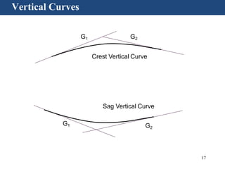
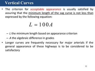
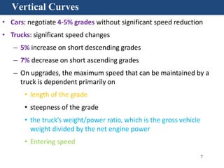
Vertical curves are used in highway design to gradually transition between two different slopes or grades. There are two main types - crest vertical curves, which are used on roadway tops, and sag vertical curves, which are used on dips. The minimum length of a vertical curve is determined based on providing the required stopping sight distance for a given design speed. Additional criteria like passenger comfort, drainage, and appearance may also influence the curve length selected. Longer vertical curves generally provide a smoother ride but require more construction costs.

1. Alignment Of Highways
1
Vertical Curves
Transportation Engineering
(CE-421)

2. 2
Vertical Curves
• Vertical alignment: specifies the
elevations of points along a
roadway
• Need to find elevation of
roadway points:
– to provide proper drainage
– an acceptable level of driver
safety/ comfort

3. 3
Vertical Curves
• A primary concern in vertical alignment: is establishing the
transition of roadway elevations between two grades
• This transition is achieved by means of vertical curves
• Broadly classification of vertical curves:
– crest vertical curves
– sag vertical curves

4. 4
Vertical Curves
• Factors influencing the vertical alignment of a highway:
– Natural terrain
– Minimum stopping sight distance for the selected design speed
– The number of trucks and other heavy vehicles in the traffic
stream
– The basic roadway cross-section; i.e., two lanes versus multiple
lanes
– Natural environmental factors, such as wetlands and historic,
cultural, and community resources

5. 5
Vertical Curves
o When grade is expressed as a percent, the grade indicates the
relative rise (or fall) of the facility in the longitudinal direction as a
percentage of the length of the section under study
o Thus, a 4% grade of 2,000 ft. involves a vertical rise of
2,000* (4/100) = 80 ft.
o Upgrades have positive slopes and percent grades, while
o downgrades have negative slopes and percent grades

6. 6
Vertical Curves
o Maximum recommended grades depend upon the :
 type of facility (road functional class)
 terrain in which it is built
 design speed
o Terrain Classification
– Level - highway sight distances are long without major expense,
small amounts of earthwork
– Rolling - the natural slopes rise above or fall below the road
elevation with occasional steep slopes that restrict highway
alignment, moderate amounts of earthwork
– Mountainous - highway alignment is strongly influenced by the
ground slopes, large amount of earthwork

7. 7
Vertical Curves
• Cars: negotiate 4-5% grades without significant speed reduction
• Trucks: significant speed changes
– 5% increase on short descending grades
– 7% decrease on short ascending grades
– On upgrades, the maximum speed that can be maintained by a
truck is dependent primarily on
• length of the grade
• steepness of the grade
• the truck’s weight/power ratio, which is the gross vehicle
weight divided by the net engine power
• Entering speed

8. 8
Vertical Curves
Source:AASHTO’s 'A Policy on Geometric Design of Highways and Streets (2011) '

9. 9
Vertical Curves
Source:AASHTO’s 'A Policy on Geometric Design of Highways and Streets (2011) '

10. 10
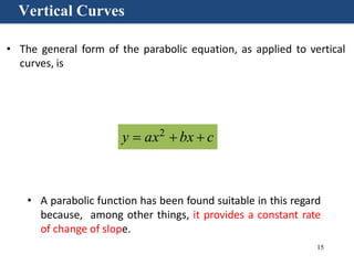
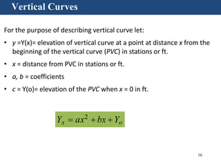
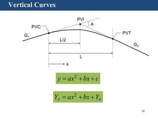
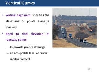
Vertical Curves
• Maximum grades:
– 5 % for a design speed of 110 km/h [70 mph]
– 7 to 12% for a design speed of 50 km/h [30 mph] depending on
terrain
• Minimum grades:
– Flat grades can typically provide proper surface drainage on
uncurbed highways where the cross slope is adequate to drain the
pavement surface laterally
– With curbed highways or streets, longitudinal grades should be
provided to facilitate surface drainage
– An appropriate minimum grade is typically 0.5 percent, but grades
of 0.30 percent may be used

11. 11
Vertical Curves
Grades

12. 12
Vertical Curves
Critical Lengths of Grade for Design
The term “critical length of grade” is used to
indicate the maximum length of a designated upgrade
on which a loaded truck can operate without an
unreasonable reduction in speed.
If the desired freedom of operation is to be
maintained on grades longer than critical, design
adjustments such as changes in location to reduce
grades or addition of extra lanes should be considered.

13. 13
Vertical Curves
*Based on accident Involvement rates with
10 mph speed reduction as threshold.

14. 14
Vertical Curves
• a 3% grade causes a reduction in speed of 10 mph after 1600 feet
1800-ft

15. 15
Vertical Curves
• The general form of the parabolic equation, as applied to vertical
curves, is
• A parabolic function has been found suitable in this regard
because, among other things, it provides a constant rate
of change of slope.
y  ax2
 bx  c

16. 16
Vertical Curves
For the purpose of describing vertical curve let:
• y =Y(x)= elevation of vertical curve at a point at distance x from the
beginning of the vertical curve (PVC) in stations or ft.
• x = distance from PVC in stations or ft.
• a, b = coefficients
• c = Y(o)= elevation of the PVC when x = 0 in ft.
Yx  ax2
 bx Yo

17. 17
Vertical Curves
G1 G2
G1 G2
Crest Vertical Curve
Sag Vertical Curve

18. 18
Vertical Curves
G1
G2
PVI
PVT
PVC
L/2
A
L
x
y  ax2
 bx  c
Yx  ax2
 bx Yo

19. Vertical Curves
Fundamentalso In defining a and b, the first derivative of equation (1) gives the slope as:
𝒅𝒀
𝒅𝒙
= 𝟐𝒂𝒙 + 𝒃
o At the PVC, x = 0, so, 𝒃 = 𝒅𝒀
= 𝑮 𝟏 (when X=0, slope is equal to entry grade)
𝒅𝒙
o where G1 is the initial slope in ft./ft.
o Also the second derivative of equation (1) is the rate of change of slope and is
𝒅 𝟐 𝒀
= 𝟐𝒂
𝒅𝒙 𝟐
o However, the average rate of change of slope, by observation (previous figure),
can also be written as
𝒅 𝟐 𝒀 𝑮 𝟐 − 𝑮 𝟏
𝒅𝒙 𝟐 =
𝑳
o Equating two equations we get
𝒂 =
𝑮 𝟐 − 𝑮 𝟏
𝟐𝑳
o Where: L – curve length in ft., G1– initial grade in ft./ft. and G2– final grade in
ft./ft.
2
19
 (1)x oY  ax  bx Y
Vertical CurvesVertical Curves

20. 20
Vertical Curves

21. 21
Vertical Curves
Example: A crest vertical curve joins a +3% and –4% grade. Design
speed is 75 mph. Length = 2184.0 ft. Station at VPI is 345+ 60.00,
elevation at VPI = 250 feet. Find elevations and station for VPC and VPT.

22. 22
Vertical Curves
Minimum lengths of crest vertical
curves based on sight distance criteria
generally are satisfactory from the
standpoint of
• Safety
• Comfort
• appearance.

23. Vertical Curve
Design• Provision of a minimum stopping sight distance (SSD) is the only
criterion used for design of a crest vertical curve
• Sight distance is measured from an assumed eye height of 3.5 ft.
and an object height of 2.0 ft.
• For crest vertical curves, the daylight sight line controls minimum
length of vertical curves
23

24. Vertical Curve
Design• Two possible scenarios that could control the design length:
– (1) the SSD is greater than the length of the vertical curve
– (2) the SSD is less than the length of the vertical curve
24

25. Vertical Curve
Design
Assistant with Target Rod (2ft object height)
Observer with Sighting
Rod (3.5 ft)
25

26. 2158
26
ASSD2
L 
A

2158
L  2SSD
For SSD/ S/ d(s) < L For SSD / S/ d(s) >L
Minimum Length of Crest Vertical Curve Design
• Longer curve lengths provide more SSD all else being equal, but more costly
to construct
• Shorter curve lengths are less expensive to construct but may not provide
adequate SSD due to more rapid changes in slope
• Requirement: An expression for minimum curve length given a required
SSD for crest vertical curve
• SSD = stopping sight distance in ft (m), and
• A = algebraic difference in grades in percent
• L = minimum length of vertical curve in ft

27. Vertical Curve Design
27

28. 28
Vertical Curves
At least four different criteria for establishing
lengths of sag vertical curves are recognized to
some extent. These are
• Headlight sight distance,
• Passenger comfort,
• Drainage control, and
• General appearance.

29. 29
Vertical Curves
• The headlight SSD requirement is based on the fact that sight distance will be
restricted during periods of darkness whereas during daylight periods, sight
distance is unaffected by the sag curve
• As a vehicle is driven on a sag vertical curve at night, the position of the
headlight and the direction of the headlight beam will dictate the stretch of
highway ahead that is lighted
• Assumptions for design (AASHTO)
– h1 = headlight height = 2.0ft.
– β = 1 degree (inclined angle of the headlight beam
relative to the horizontal
plan of the car)

30. Vertical Curves
G1
G2
PVI
PVTPVC
h2=0h1
L
Light Beam Distance =(S)
For SSD < L
For SSD > L
headlight beam (diverging from LOS by β degrees)
ASSD2
30
L 
4003.5SSD 
 A
 4003.5SSD
L  2SSD
D

31. 31
Vertical Curves
• The comfort criterion is based on the fact that when a vehicle travels on a sag
vertical curve, both the gravitational and centrifugal forces act in combination,
resulting in a greater effect than on a crest vertical curve where these forces act in
opposition to each other
• Several factors such as weight carried, body suspension of the vehicle, and tire
flexibility affect comfort due to change in vertical direction, making it difficult for
comfort to be measured directly
• It is generally accepted that a comfortable ride will be provided if the radial
acceleration is not greater than 1 ft /sec-sq.
• Minimum length of curve
– where V is the design speed in mph
– L the minimum length based on comfort
– A the algebraic difference in grades

32. 32
Vertical Curves
• The criterion for acceptable appearance is usually satisfied by
assuring that the minimum length of the sag curve is not less than
expressed by the following equation:
L  100A
– L the minimum length based on appearance criterion
– A the algebraic difference in grades
• Longer curves are frequently necessary for major arterials if the
general appearance of these highways is to be considered to be
satisfactory

33. 33
Vertical Curves
Length of Sag Vertical Curves Based on Drainage Criterion
• The drainage criterion for sag vertical curves must be
considered when the road is curbed
• This criterion is different from the others in that there is a
maximum length requirement rather than a minimum
length
• The maximum length requirement to satisfy the drainage
criterion is that a minimum slope of 0.35 percent be
provided within 50 ft. of the lowest point of the curve

34. Additional Properties of Vertical Curves
32
o G1 = initial roadway grade in percent or ft/ft (m/m) (this grade is also
referred to as the initial tangent grade(viewing from left to right)
o G2 = final roadway (tangent) grade in percent or ft/ft(m/m),
o PVC = point of the vertical curve (the initial point of the curve),
o PVI = point of vertical intersection (intersection of initial and final grades),
o PVT = point of vertical tangent, which is the final point of the vertical curve
(the point where the curve returns to the final grade or, equivalently, the
final tangent),

35. Additional Properties of Vertical Curves
o L = length of the curve in stations or ft (m) measured in a constant-
elevation horizontal plane,
o x =
o Y =
distance from the PVC in ft (m),
offset at any distance x from the PVC in ft (m),
o Ym = mid-curve offset in ft (m), and
o Yf= offset at the end of the vertical curve in ft (m).
o Making use of the properties of an equal-tangent parabola
o Where A = absolute value of the difference in grades (|G1 - G2|)
expressed in percent
x2
35
A
200L
Y 

36. Additional Properties of Vertical Curves
o Mid-curve offset
o Offset at the end of curve
o Note that in this equation, 200 is used in the denominator insteadof
2 because A is expressed in percent instead of ft/ft
o The K-value defined as (with L in ft and A in percent)
o K = value that is the horizontal distance, in ft. required to affect a
1% change in the slope of the vertical curve,
o A = absolute value of the difference in grades (|G1  G2|)
expressed in percent), and
o L = length of curve in ft (m).
A L
8 0 0
mY 
A L
2 0 0fY 
K 
L
A
36