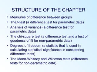
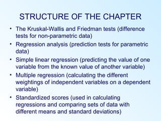
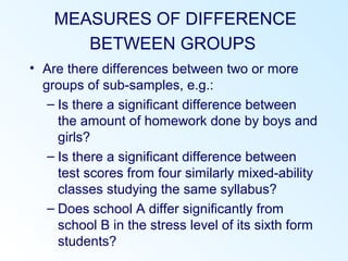
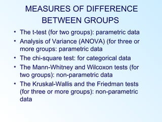
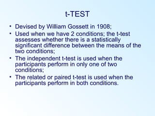
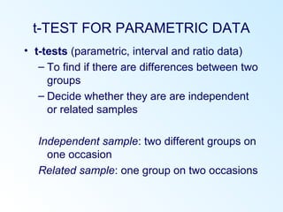
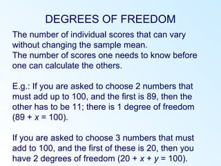
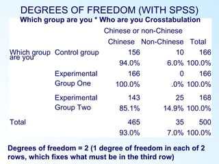
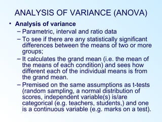
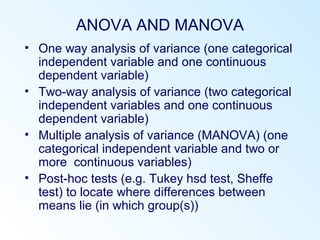
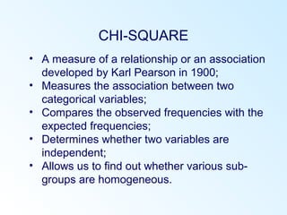
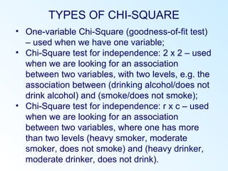
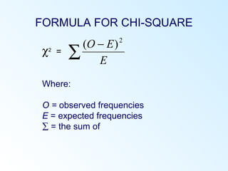
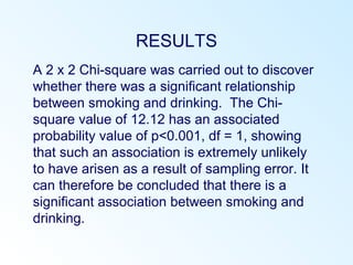
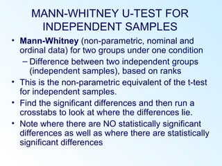
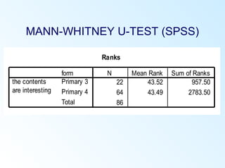
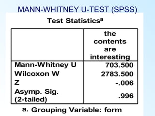
SlideShare a Scribd company logo
INFERENTIAL STATISTICS
© LOUIS COHEN, LAWRENCE
MANION & KEITH MORRISON
STRUCTURE OF THE CHAPTER
• Measures of difference between groups
• The t-test (a difference test for parametric data)
• Analysis of variance (a difference test for
parametric data)
• The chi-square test (a difference test and a test of
goodness of fit for non-parametric data)
• Degrees of freedom (a statistic that is used in
calculating statistical significance in considering
difference tests)
• The Mann-Whitney and Wilcoxon tests (difference
tests for non-parametric data)
STRUCTURE OF THE CHAPTER
• The Kruskal-Wallis and Friedman tests (difference
tests for non-parametric data)
• Regression analysis (prediction tests for parametric
data)
• Simple linear regression (predicting the value of one
variable from the known value of another variable)
• Multiple regression (calculating the different
weightings of independent variables on a dependent
variable)
• Standardized scores (used in calculating
regressions and comparing sets of data with
different means and standard deviations)
MEASURES OF DIFFERENCE
BETWEEN GROUPS
• Are there differences between two or more
groups of sub-samples, e.g.:
– Is there a significant difference between
the amount of homework done by boys and
girls?
– Is there a significant difference between
test scores from four similarly mixed-ability
classes studying the same syllabus?
– Does school A differ significantly from
school B in the stress level of its sixth form
students?
MEASURES OF DIFFERENCE
BETWEEN GROUPS
• The t-test (for two groups): parametric data
• Analysis of Variance (ANOVA) (for three or
more groups: parametric data
• The chi-square test: for categorical data
• The Mann-Whitney and Wilcoxon tests (for
two groups): non-parametric data
• The Kruskal-Wallis and the Friedman tests
(for three or more groups): non-parametric
data
t-TEST
• Devised by William Gossett in 1908;
• Used when we have 2 conditions; the t-test
assesses whether there is a statistically
significant difference between the means of the
two conditions;
• The independent t-test is used when the
participants perform in only one of two
conditions;
• The related or paired t-test is used when the
participants perform in both conditions.
t-TEST FOR PARAMETRIC DATA
• t-tests (parametric, interval and ratio data)
– To find if there are differences between two
groups
– Decide whether they are are independent
or related samples
Independent sample: two different groups on
one occasion
Related sample: one group on two occasions
t-TEST FOR PARAMETRIC DATA
Formula for computing the t-test
Sample one mean – sample two mean
t = 
Standard error of the difference in means
Formula for calculating t














+







−+
+
−
=
∑ ∑
2121
2
2
2
1
21
11
2 NNNN
dd
MM
t
M = Mean
d = difference between the means
N = Number of cases
t-TEST FOR INDEPENDENT SAMPLES
The t-test computes a ratio between a measure of
the between-groups variance and the within group
variance.
The larger the variance between the groups
(columns), compared with the variance within the
groups (rows), the larger the t-value.
INDEPENDENT AND RELATED
SAMPLES IN A t-TEST: EXAMPLES
1. Independent sample (two groups):
• A group of scientists wants to study the effects of a
new drug for insomnia. They have applied this drug to
a random group of people (control group) and to a
group of people suffering from insomnia (experimental
group);
1. Related sample (same group in two conditions):
• A group of therapists wants to study whether there is
any difference in doing relaxation techniques on the
beach or in an apartment. A group of people is asked
to first do relaxation on the beach and later in an
apartment;
INDEPENDENT AND RELATED
SAMPLES IN A t-Test: AN EXAMPLE
24 people were involved in an experiment to
determine whether background noise affects
short-term memory (recall of words);
– If half of the sample were allocated to the
NOISE condition and the other half to the
NO NOISE condition (independent
sample) – we use independent t-test;
– If everyone in the sample has performed at
both conditions (related sample) – we use
paired or related t-test.
AN EXAMPLE OF A t-TEST
Participants were asked to memorize a list of 20
words in two minutes.
Half of the sample performs in a noisy environment
and the other half in a quiet environment;
Independent variable - two types of environment:
Quiet environment (NO NOISE condition)
Noisy environment (NOISE condition)
Dependent variable – the number of words each
participant can recall.
NOISE NO NOISE
5 15
10 9
6 16
6 15
7 16
3 18
6 17
9 13
5 11
10 12
11 13
9 11
Σ = 87 Σ = 166
= 7.3 = 13.8
SD = 2.5 SD = 2.8
XX
NOTE: participants vary within
conditions: in the NOISE condition,
the scores range from 3 to 11, and in
the NO NOISE condition. They range
from 9 to 18;
The participants differ between the
conditions too: the scores of the NO
NOISE condition, in general, are
higher than those in the NOISE
condition – the means confirm it;
Are the differences between the
means of our groups large enough for
us to conclude that the differences are
due to our independent variable:
NOISE/NO NOISE manipulation?
t-TEST FOR INDEPENDENT SAMPLES
Group statistics
In which condition
are you? N Mean Std. Deviation
Std. Error
Mean
How many words
can you recall?
NOISE 12 7.2500 .71906
NO NOISE 12 13.8333 .79614
This shows:
the name of 2 conditions;
the number of cases in each condition;
the mean of each condition;
the standard deviation and standard error of
the mean, of the two conditions.
t-TEST FOR INDEPENDENT SAMPLES (SPSS)
Independent Samples Test
Levene’s Test
for Equality of
Variances t-test for Equality of Means
F Sig t df
Sig.
(2-tailed)
Mean
Differences
Std. Error
Differences
95%
Confidence
Interval of the
Difference
Lower Upper
How many
words can
you recall?
Equal variances
assumed
.177 .676 -6.137 22 .000 -6.5833 1.07279 -8.808 -4.359
Equal variances
not assumed
-6.137 21.78 .000 -6.5833 1.07279 -8.809 -4.357
The Levene test is for ‘homogeneity of variance’,
and the t-test here indicates whether you should
use the upper or lower row.
Mean Difference means the difference between the
means of the two groups.
REPORTING FINDINGS FROM THE
EXAMPLE
Participants in the NOISE condition recalled fewer
words (t (22) = 7.25, SD = 2.49) than in the NO
NOISE condition (t (22) = 13.83, SD = 2.76). The
mean difference between conditions was 6.58; the
95% confidence interval for the estimated population
mean difference is between 4.36 and 8.81. An
independent t-test revealed that, if the null
hypothesis is true, such a result would be highly
unlikely to have arisen (t (22) = 6.14; p<0.001). It is
therefore concluded that listening to noise affects
short-term memory, at least in respect of word recall.
Group Statistics
Which group are you N Mean
Std.
Deviation
Std. Error
Mean
Mathematics post-test
score
Control group 166 8.69 1.220 .095
Experimental Group One 166 9.45 .891 .069
t-TEST FOR INDEPENDENT
SAMPLES WITH SPSS
Read the line ‘Levene’s Test for Equality of Variances’. If the
probability value is statistically significant then your variances
are unequal; otherwise they are regarded as equal. If the
Levene’s probability value is not statistically significant then
you need the row ‘equal variances assumed’; if the Levene’s
probability value is statistically significant then you need the
row ‘equal variances not assumed’. Look to the column ‘Sig.
(2-tailed)’ and the appropriate row, and see if the results are
statistically significant.
Independent Samples Test
Levene's Test for
Equality of
Variances t-test for Equality of Means
95% Confidence
Interval of the
Difference
F Sig. t df
Sig. (2-
tailed)
Mean
Difference
Std. Error
Difference Lower Upper
Mathematics
post-test score
Equal variances
assumed
28.856 .000 -6.523 330 .000 -.765 .117 -.996 -.534
Equal variances
not assumed
-6.523 302.064 .000 -.765 .117 -.996 -.534
PAIRED SAMPLE t-TEST (SAME GROUP
UNDER TWO CONDITIONS) WITH SPSS
Paired Samples Statistics
Mean N
Std.
Deviation
Std. Error
Mean
Pair 1 Mathematics pre-test
score
6.95 252 1.066 .067
Mathematics post-test
score
8.94 252 1.169 .074
This indicates:
1.The two conditions;
2.The mean of each condition;
3.The number of cases in each condition;
4.The standard deviation and standard error of the
mean, for the two conditions.
PAIRED SAMPLE t-TEST (SAME GROUP
UNDER TWO CONDITIONS) WITH SPSS
This shows that there is no association between the
scores on the pre-test and the scores on the post
test for the group in question (r = .02 and ρ = .749).
Paired Samples Correlations
N Correlation Sig.
Pair 1 Mathematics pre-test
score & Mathematics
post-test score
252 .020 .749
PAIRED SAMPLE t-TEST (SAME GROUP UNDER
TWO CONDITIONS) WITH SPSS
This shows that :
1.The difference between the mean of each condition (6.95 and
8.94) is 1.992.
2.The confidence intervals shows that we are 95% certain that the
population difference lies somewhere between -2.186 and -1.798.
3.There is a statistically significant difference between the two sets
of scores.
Paired Samples Test
Paired Differences
t df
Sig.
(2-tailed)Mean
Std.
Deviation
Std.
Error
Mean
95%
Confidence
Interval of the
Difference
Lower Upper
Pair
1
Mathematics
pre-test score -
Mathematics
post-test score
-1.992 1.567 .099 -2.186 -1.798 -20.186 251 .000
RESULT
It can be seen from the paired t-test that the
hypothesis is not supported (t (251) = 20.186;
ρ=.000).
DEGREES OF FREEDOM
The number of individual scores that can vary
without changing the sample mean.
The number of scores one needs to know before
one can calculate the others.
E.g.: If you are asked to choose 2 numbers that
must add up to 100, and the first is 89, then the
other has to be 11; there is 1 degree of freedom
(89 + x = 100).
If you are asked to choose 3 numbers that must
add to 100, and the first of these is 20, then you
have 2 degrees of freedom (20 + x + y = 100).
DEGREES OF FREEDOM (WITH SPSS)
Which group are you * Who are you Crosstabulation
Chinese or non-Chinese
TotalChinese Non-Chinese
Which group
are you
Control group 156 10 166
94.0% 6.0% 100.0%
Experimental
Group One
166 0 166
100.0% .0% 100.0%
Experimental
Group Two
143 25 168
85.1% 14.9% 100.0%
Total 465 35 500
93.0% 7.0% 100.0%
Degrees of freedom = 2 (1 degree of freedom in each of 2
rows, which fixes what must be in the third row)
ANALYSIS OF VARIANCE (ANOVA)
• Analysis of variance
– Parametric, interval and ratio data
– To see if there are any statistically significant
differences between the means of two or more
groups;
– It calculates the grand mean (i.e. the mean of
the means of each condition) and sees how
different each of the individual means is from
the grand mean.
– Premised on the same assumptions as t-tests
(random sampling, a normal distribution of
scores, independent variable(s) is/are
categorical (e.g. teachers, students,) and one
is a continuous variable (e.g. marks on a test).
ANOVA AND MANOVA
• One way analysis of variance (one categorical
independent variable and one continuous
dependent variable)
• Two-way analysis of variance (two categorical
independent variables and one continuous
dependent variable)
• Multiple analysis of variance (MANOVA) (one
categorical independent variable and two or
more continuous variables)
• Post-hoc tests (e.g. Tukey hsd test, Sheffe
test) to locate where differences between
means lie (in which group(s))
( )
( )
( )groupsN
groups
mean
df
d
varianceWithin
df
NXd
ancevariBetween
variancegroups-within
variancegroups-between
atiorF
−
−
∑
∑
=
=
=
2
1
2
FORMULA FOR ANOVA
Between-groups and within-groups variance:
Variation between the groups (9 to 22.2);
Variation within the first group (no variation since all
participants scored the same);
Variation within the second group (from 15 to 16);
Variation within the third group (from 17 to 26).
A1 A2 A3
9 15 21
9 15 25
9 16 17
9 15 22
9 16 26
= 9 = 15.4 = 22.2X X X
ANOVA
1. First, ANOVA calculates the mean for each of
the three groups;
2. Then it calculates the grand mean (the three
means added then divided by three);
3. For each group separately, the total deviation of
each individual’ s score from the mean of the
group is calculated (within-groups variation);
4. Then the deviation of each group mean from the
grand mean is calculated (between-groups
variation).
F RATIO
When we conduct our experiment, we hope that the
between-groups variance is very much larger than the
within-groups variance, in order to get a bigger F ratio;
This shows us that one (or more) of the individual
group means is significantly different from the grand
mean;
However, it does not tell us which means are
statistically significantly different.
cevarianroupsg-within
variancegroups-between
ratioF =
Descriptives
Records of students' progress
7 3.29 .76 .29 2.59 3.98 2 4
5 3.80 1.30 .58 2.18 5.42 2 5
4 3.25 .96 .48 1.73 4.77 2 4
1 4.00 . . . . 4 4
17 3.47 .94 .23 2.99 3.96 2 5
20-29
30-39
40-49
50+
Total
N Mean
Std.
Deviation
Std.
Error Lower Bound Upper Bound
95% Confidence Interval for
Mean
Minimum Maximum
ANOVA
Records of students' progress
1.257 3 .419 .420 .742
12.979 13 .998
14.235 16
Between Groups
Within Groups
Total
Sum of
Squares df Mean Square F Sig.
Between-groups
variation
Within-groups
variation
F (3,13) = .420, ρ=.742
RESULTS
An F ratio of .420 has been given, with a
probability of ρ=.742. This tells us that there
is no statistically significant difference
between any of the groups.
EFFECT SIZE: PARTIAL ETA SQUARED
erroreffect
effect
partial
SSSS
SS
squaredetaPartial
+
=)( 2
η
SSeffect = The sums of the squares for whatever
effect is of interest;
SSerror = the sums of the squares for whatever
error term is associated with that effect.
EFFECT SIZE: PARTIAL ETA SQUARED FOR
INDEPENDENT SAMPLES IN SPSS
Analyze → General Linear Model → Univariate →
Options → Estimates of effect size
Between-Subjects Factors
Value Label N
Which group are you 1 Control group 166
2 Experimental Group One 166
3 Experimental Group Two 168
EFFECT SIZE: PARTIAL ETA SQUARED
IN SPSS
EFFECT SIZE: PARTIAL ETA
SQUARED IN SPSS
Tests of Between-Subjects Effects
Dependent Variable:Mathematics post-test score
Source
Type III
Sum of
Squares df Mean Square F Sig.
Partial Eta
Squared
Corrected Model 48.583a
2 24.291 23.168 .000 .085
Intercept 41113.093 1 41113.093 39211.30
1
.000 .987
group 48.583 2 24.291 23.168 .000 .085
Error 521.105 497 1.049
Total 41684.000 500
Corrected Total 569.688 499
a. R Squared = .085 (Adjusted R Squared = .082)
THE POST HOC TUKEY TEST
• The null hypothesis for the F-test ANOVA is
always that the samples come from populations
with the same Mean (i.e., no statistically
significant differences): H0 = μ1 = μ2 = μ3 = …
• If the p-value is so low that we reject the null
hypothesis, we have decided that, at least one of
these populations has a mean that is not equal to
the others;
• The F-test itself only tells us that there are
differences at least between one pair of means,
not where these differences lie.
POST HOC TESTS
• To determine which samples are statistically
significantly different; after having performed the
F-test and rejected the null hypothesis, we turn
to post hoc comparisons;
• The purpose of a post hoc analysis is to find out
exactly where those differences are;
• Post hoc tests allow us to make multiple pair
wise comparisons and determine which pairs are
statistically significantly different from each other
and which are not.
THE POST HOC TUKEY TEST
Tukey’s Honestly Significant Difference (HSD)
Test is used to test the hypothesis that all
possible pairs of means are equal;
Tukey’s HSD test compares the mean
differences between each pair of means to a
critical value. If the mean difference from a pair
of means exceeds the critical value, we
conclude that there is a significant difference
between these pairs.
THE SCHEFFE TEST
The Scheffe test is very similar to the Tukey
hsd test, but it is more stringent that the Tukey
test in respect of reducing the risk of a Type I
error, though this comes with some loss of
power – one may be less likely to find a
difference between groups in the Sheffe test.
FINDING PARTIAL ETA SQUARED IN SPSS
Multivariate Testsb
Effect Value F
Hypothesis
df Error df Sig.
Partial Eta
Squared
scores Pillai's Trace .675 1033.477a
1.000 497.000 .000 .675
Wilks' Lambda .325 1033.477a
1.000 497.000 .000 .675
Hotelling's Trace 2.079 1033.477a
1.000 497.000 .000 .675
Roy's Largest Root 2.079 1033.477a
1.000 497.000 .000 .675
scores *
group
Pillai's Trace .040 10.366a
2.000 497.000 .000 .040
Wilks' Lambda .960 10.366a
2.000 497.000 .000 .040
Hotelling's Trace .042 10.366a
2.000 497.000 .000 .040
Roy's Largest Root .042 10.366a
2.000 497.000 .000 .040
a. Exact statistic
b. Design: Intercept + group
Within Subjects Design: scores
USING TUKEY TO LOCATE
DIFFERENCE IN SPSS
Multiple Comparisons
MEASURE_1
Tukey HSD
(I) Which
group are you (J) Which group are you
Mean
Difference
(I-J)
Std.
Error Sig.
95% Confidence
Interval
Lower
Bound
Upper
Bound
Control group Experimental Group One -.42*
.084 .000 -.61 -.22
Experimental Group Two -.15 .084 .173 -.35 .05
Experimental
Group One
Control group .42*
.084 .000 .22 .61
Experimental Group Two .27*
.084 .005 .07 .46
Experimental
Group Two
Control group .15 .084 .173 -.05 .35
Experimental Group One -.27*
.084 .005 -.46 -.07
Based on observed means.
The error term is Mean Square(Error) = .588.
*. The mean difference is significant at the .05 level.
USING TUKEY TO LOCATE DIFFERENCE IN SPSS
MEASURE_1
Tukey HSDa,,b,,c
Which group are you N
Subset
1 2
Control group 166 7.86
Experimental Group Two 168 8.01
Experimental Group One 166 8.27
Sig. .174 1.000
Means for groups in homogeneous subsets are displayed.
Based on observed means.
The error term is Mean Square(Error) = .588.
a. Uses Harmonic Mean Sample Size = 166.661.
b. The group sizes are unequal. The harmonic mean of the
group sizes is used. Type I error levels are not guaranteed.
c. Alpha = .05.
CHI-SQUARE
• A measure of a relationship or an association
developed by Karl Pearson in 1900;
• Measures the association between two
categorical variables;
• Compares the observed frequencies with the
expected frequencies;
• Determines whether two variables are
independent;
• Allows us to find out whether various sub-
groups are homogeneous.
TYPES OF CHI-SQUARE
• One-variable Chi-Square (goodness-of-fit test)
– used when we have one variable;
• Chi-Square test for independence: 2 x 2 – used
when we are looking for an association
between two variables, with two levels, e.g. the
association between (drinking alcohol/does not
drink alcohol) and (smoke/does not smoke);
• Chi-Square test for independence: r x c – used
when we are looking for an association
between two variables, where one has more
than two levels (heavy smoker, moderate
smoker, does not smoke) and (heavy drinker,
moderate drinker, does not drink).
FORMULA FOR CHI-SQUARE
χ2
=
Where:
O = observed frequencies
E = expected frequencies
∑ = the sum of
∑
−
E
EO 2
)(
ONE-VARIABLE CHI-SQUARE OR
GOODNESS-OF-FIT TEST
• Enables us to discover whether a set of obtained
frequencies differs from an expected set of
frequencies;
• One variable only;
• The numbers that we find in the various
categories are called the observed frequencies;
• The numbers that we expect to find in the
categories, if the null hypothesis is true, are the
expected frequencies;
• Chi-Square compares the observed and the
expected frequencies.
EXAMPLE: PREFERENCE FOR
CHOCOLATE BARS
A sample of 120 people were asked which of
four chocolate bars they preferred;
• We want to find out whether some brands (or
one brand) are preferred over others –
Research Hypothesis;
• If some brands are not preferred over others,
then all brands should be equally represented
– Null Hypothesis;
• If the Null Hypothesis is true, then we expect
30 (120/4) people in each category
ONE-VARIABLE CHI-SQUARE OR
GOODNESS-OF-FIT TEST
If all brands of chocolate are equally popular, the
observed frequencies will not differ much from the
expected frequencies;
If, however, the observed frequencies differ a lot
from the expected frequencies, then it is likely that
all brands are not equally popular;
Frequencies Chocolate A Chocolate B Chocolate C Chocolate D
Observed 20 70 10 20
Expected 30 30 30 30
ONE-VARIABLE CHI-SQUARE/GOODNESS-
OF-FIT TEST
Observed
N
Expected
N
Residual
(Difference between
observed and expected
frequencies)
Brand A 20 30 -10.0
Brand B 70 30 40.0
Brand C 10 30 -20.0
Brand D 20 30 -10.0
Total 120 120
Chocolate
Chi-square
df
Asymp.
Sig
73.333
3
.000
A chi-square value of 73.3, df = 3 was found to
have an associated probability level of 0.000. A
statistically significant difference was found
between the observed and the expected
frequencies, i.e. all brands of chocolate are not
equally popular. More people prefer chocolate B
(70) than the other bars of chocolate.
CHI-SQUARE TEST FOR
INDEPENDENCE (BIVARIATE): 2 X 2
Enables us to discover whether there is a
relationship or association between two
categorical variables of 2 levels;
If there is no association between the two
variables, then we conclude that the variables
are independent of each other.
A WORKED EXAMPLE
Imagine that we have asked 110 students the
following:
A. Do you smoke and drink?
B. Do you smoke but do not drink?
C. Do you not smoke but drink?
D. Do you abstain from both?
Each student can only fall into one group, and
thus we have 4 groups (they must be
mutually exclusive);
CHI-SQUARE TEST FOR
INDEPENDENCE: 2 X 2 (WITH SPSS)
Do you drink? * Do you smoke? Crosstabulation
Do you smoke?
Yes No Total
Do you
drink? Yes Count 50 15 65
Expected Count 41.4 23.6 65.0
No Count 20 25 45
Expected Count 28.6 16.4 45.0
Total Count 70 40 110
Expected Count 70.0 40.0 110.0
totalOverall
totalcolumnxtotalrow
cellaofvalueExpected =
CHI-SQUARE TEST FOR
INDEPENDENCE: 2 X 2 (WITH SPSS)
Value df Asymp. Sig. Exact Sig.
(2-sided)
Exact Sig.
(1-sided)
Pearson Chi-Square 12.12 1 .000
Continuity Correction 10.759 1 .001
Likelihood Ratio 12.153 1 .001
Fisher’s Exact Test .001 .001
Linear-by-Linear
Association
12.011 1 .001
N of Valid Cases 110
Chi-Square = 12.12
df (degrees of freedom) = (columns -1) x (rows -1)
= (2-1) x (2-1) = 1
RESULTS
A 2 x 2 Chi-square was carried out to discover
whether there was a significant relationship
between smoking and drinking. The Chi-
square value of 12.12 has an associated
probability value of p<0.001, df = 1, showing
that such an association is extremely unlikely
to have arisen as a result of sampling error. It
can therefore be concluded that there is a
significant association between smoking and
drinking.
MANN-WHITNEY U-TEST FOR
INDEPENDENT SAMPLES
• Mann-Whitney (non-parametric, nominal and
ordinal data) for two groups under one condition
– Difference between two independent groups
(independent samples), based on ranks
• This is the non-parametric equivalent of the t-test
for independent samples.
• Find the significant differences and then run a
crosstabs to look at where the differences lie.
• Note where there are NO statistically significant
differences as well as where there are statistically
significant differences
MANN-WHITNEY U-TEST (SPSS)
Ranks
22 43.52 957.50
64 43.49 2783.50
86
form
Primary 3
Primary 4
Total
the contents
are interesting
N Mean Rank Sum of Ranks
Test Statisticsa
703.500
2783.500
-.006
.996
Mann-Whitney U
Wilcoxon W
Z
Asymp. Sig.
(2-tailed)
the
contents
are
interesting
Grouping Variable: forma.
MANN-WHITNEY U-TEST (SPSS)
THE WILCOXON TEST FOR RELATED
SAMPLES
This is the non-parametric equivalent of the t-test
for related samples.
For paired (related) samples in a non-parametric
test, e.g. the same group under two conditions.
For example, here is the result for one group of
females who have rated (a) their own ability in
mathematics and (b) their enjoyment of
mathematics, both variables using a 5-point scale
(‘not at all’ to ‘a very great deal’).
THE WILCOXON TEST FOR RELATED SAMPLES (SPSS)
Test Statisticsb
How good at mathematics do you
think you are? - How much do you
enjoy mathematics?
Z -2.631a
Asymp. Sig. (2-tailed) .009
a. Based on positive ranks.
b. Wilcoxon Signed Ranks Test
Ranks
N Mean Rank Sum of Ranks
How good at
mathematics
do you think
you are? - How
much do you
enjoy
mathematics?
Negative Ranks 11 94.08 11101.00
Positive Ranks 73 99.11 7235.00
Ties 57
Total 248
KRUSKAL-WALLIS TEST FOR
INDEPENDENT SAMPLES
• Kruskal-Wallis (non-parametric, nominal and
ordinal data) for three or more independent groups
under one condition
– Difference between more than two independent
groups (independent samples), based on ranks
• This is the non-parametric equivalent of ANOVA
for independent samples.
• Find the statistically significant differences and
then run a crosstabs to look at where the
differences lie.
• Note where there are NO statistically significant
differences as well as where there are statistically
significant differences.
Ranks
7 6.57
5 10.70
5 10.70
17
Age
20-29
30-39
40-49
Total
own made-up tests
N Mean Rank
KRUSKAL-WALLIS TEST (SPSS)
Test Statisticsa,b
4.319
2
.115
Chi-Square
df
Asymp. Sig.
own made-up
tests
Kruskal Wallis Testa.
Grouping Variable: Ageb.
KRUSKAL-WALLIS TEST (SPSS)
THE FRIEDMAN TEST FOR 3 OR MORE
RELATED GROUPS
This is the non-parametric equivalent of ANOVA for
related samples.
For three or more related samples in a non-parametric
test, e.g. the same groups under two conditions. For
example, the result for 4 groups of students, grouped
according to their IQ (Group 1= IQ up to 90; Group 2 =
IQ from 91-110; Group 3 = IQ from 111-125; Group 4 =
IQ over 125) who have rated (a) their own ability in
mathematics and (b) their enjoyment of mathematics,
both variables using a 5-point scale (‘not at all’ to ‘a
very great deal’).

More Related Content

What's hot

non parametric statistics
non parametric statisticsnon parametric statistics
non parametric statisticsAnchal Garg
 
Time Series Analysis: Theory and Practice
Time Series Analysis: Theory and PracticeTime Series Analysis: Theory and Practice
Time Series Analysis: Theory and PracticeTetiana Ivanova
 
T test, independant sample, paired sample and anova
T test, independant sample, paired sample and anovaT test, independant sample, paired sample and anova
T test, independant sample, paired sample and anovaQasim Raza
 
Chi-square, Yates, Fisher & McNemar
Chi-square, Yates, Fisher & McNemarChi-square, Yates, Fisher & McNemar
Chi-square, Yates, Fisher & McNemarAzmi Mohd Tamil
 
Chi square test final
Chi square test finalChi square test final
Chi square test finalHar Jindal
 
statistical estimation
statistical estimationstatistical estimation
statistical estimationAmish Akbar
 
Research methodology chi square test
Research methodology  chi square testResearch methodology  chi square test
Research methodology chi square testPriyadharshiniV11
 
Confirmatory factor analysis (cfa)
Confirmatory factor analysis (cfa)Confirmatory factor analysis (cfa)
Confirmatory factor analysis (cfa)HennaAnsari
 
Mpc 006 - 02-03 partial and multiple correlation
Mpc 006 - 02-03 partial and multiple correlationMpc 006 - 02-03 partial and multiple correlation
Mpc 006 - 02-03 partial and multiple correlationVasant Kothari
 
Basic Statistics in 1 hour.pptx
Basic Statistics in 1 hour.pptxBasic Statistics in 1 hour.pptx
Basic Statistics in 1 hour.pptxParag Shah
 
Anova lecture
Anova lectureAnova lecture
Anova lecturedoublem44
 
Simple & Multiple Regression Analysis
Simple & Multiple Regression AnalysisSimple & Multiple Regression Analysis
Simple & Multiple Regression AnalysisShailendra Tomar
 
Arima model (time series)
Arima model (time series)Arima model (time series)
Arima model (time series)Kumar P
 
Advance Statistics - Wilcoxon Signed Rank Test
Advance Statistics - Wilcoxon Signed Rank TestAdvance Statistics - Wilcoxon Signed Rank Test
Advance Statistics - Wilcoxon Signed Rank TestJoshua Batalla
 
Measurement theory.
Measurement theory.Measurement theory.
Measurement theory.ANUJA DHAKAL
 
The two sample t-test
The two sample t-testThe two sample t-test
The two sample t-testChristina K J
 
Lecture 6. univariate and bivariate analysis
Lecture 6. univariate and bivariate analysisLecture 6. univariate and bivariate analysis
Lecture 6. univariate and bivariate analysisDr Rajeev Kumar
 

What's hot (20)

non parametric statistics
non parametric statisticsnon parametric statistics
non parametric statistics
 
Time Series Analysis: Theory and Practice
Time Series Analysis: Theory and PracticeTime Series Analysis: Theory and Practice
Time Series Analysis: Theory and Practice
 
T test, independant sample, paired sample and anova
T test, independant sample, paired sample and anovaT test, independant sample, paired sample and anova
T test, independant sample, paired sample and anova
 
Correlation
CorrelationCorrelation
Correlation
 
Chi-square, Yates, Fisher & McNemar
Chi-square, Yates, Fisher & McNemarChi-square, Yates, Fisher & McNemar
Chi-square, Yates, Fisher & McNemar
 
Chi square test final
Chi square test finalChi square test final
Chi square test final
 
statistical estimation
statistical estimationstatistical estimation
statistical estimation
 
Research methodology chi square test
Research methodology  chi square testResearch methodology  chi square test
Research methodology chi square test
 
05 intervention studies
05 intervention studies05 intervention studies
05 intervention studies
 
Confirmatory factor analysis (cfa)
Confirmatory factor analysis (cfa)Confirmatory factor analysis (cfa)
Confirmatory factor analysis (cfa)
 
Anova copy
Anova   copyAnova   copy
Anova copy
 
Mpc 006 - 02-03 partial and multiple correlation
Mpc 006 - 02-03 partial and multiple correlationMpc 006 - 02-03 partial and multiple correlation
Mpc 006 - 02-03 partial and multiple correlation
 
Basic Statistics in 1 hour.pptx
Basic Statistics in 1 hour.pptxBasic Statistics in 1 hour.pptx
Basic Statistics in 1 hour.pptx
 
Anova lecture
Anova lectureAnova lecture
Anova lecture
 
Simple & Multiple Regression Analysis
Simple & Multiple Regression AnalysisSimple & Multiple Regression Analysis
Simple & Multiple Regression Analysis
 
Arima model (time series)
Arima model (time series)Arima model (time series)
Arima model (time series)
 
Advance Statistics - Wilcoxon Signed Rank Test
Advance Statistics - Wilcoxon Signed Rank TestAdvance Statistics - Wilcoxon Signed Rank Test
Advance Statistics - Wilcoxon Signed Rank Test
 
Measurement theory.
Measurement theory.Measurement theory.
Measurement theory.
 
The two sample t-test
The two sample t-testThe two sample t-test
The two sample t-test
 
Lecture 6. univariate and bivariate analysis
Lecture 6. univariate and bivariate analysisLecture 6. univariate and bivariate analysis
Lecture 6. univariate and bivariate analysis
 

Viewers also liked

Action Research Implementation
Action Research ImplementationAction Research Implementation
Action Research Implementationcfmorr
 
首尔大韩国语语法Topik考试语法合集 刘赢整理
首尔大韩国语语法Topik考试语法合集 刘赢整理首尔大韩国语语法Topik考试语法合集 刘赢整理
首尔大韩国语语法Topik考试语法合集 刘赢整理Ying Liu
 
Implementation Research: A Primer
Implementation Research: A PrimerImplementation Research: A Primer
Implementation Research: A Primeramusten
 
PS CH 10 matter properties and changes edited
PS CH 10 matter properties and changes editedPS CH 10 matter properties and changes edited
PS CH 10 matter properties and changes editedEsther Herrera
 
Test for equal variances
Test for equal variancesTest for equal variances
Test for equal variancesJohn Smith
 
NFL 2013 Combine Data Multivariate Analysis
NFL 2013 Combine Data Multivariate AnalysisNFL 2013 Combine Data Multivariate Analysis
NFL 2013 Combine Data Multivariate AnalysisJohn Michael Croft
 
Pm m23 & pmnm06 week 3 lectures 2015
Pm m23 & pmnm06 week 3 lectures 2015Pm m23 & pmnm06 week 3 lectures 2015
Pm m23 & pmnm06 week 3 lectures 2015pdiddyboy2
 
PMM23 Week 3 Lectures
PMM23 Week 3 LecturesPMM23 Week 3 Lectures
PMM23 Week 3 Lecturespdiddyboy2
 
Dte Energy Grant
Dte Energy GrantDte Energy Grant
Dte Energy Grantshoffma5
 
Univariate, bivariate analysis, hypothesis testing, chi square
Univariate, bivariate analysis, hypothesis testing, chi squareUnivariate, bivariate analysis, hypothesis testing, chi square
Univariate, bivariate analysis, hypothesis testing, chi squarekongara
 

Viewers also liked (20)

Action Research Implementation
Action Research ImplementationAction Research Implementation
Action Research Implementation
 
首尔大韩国语语法Topik考试语法合集 刘赢整理
首尔大韩国语语法Topik考试语法合集 刘赢整理首尔大韩国语语法Topik考试语法合集 刘赢整理
首尔大韩国语语法Topik考试语法合集 刘赢整理
 
Chapter4
Chapter4Chapter4
Chapter4
 
Implementation Research: A Primer
Implementation Research: A PrimerImplementation Research: A Primer
Implementation Research: A Primer
 
Ch 2 data analysis
Ch 2 data analysisCh 2 data analysis
Ch 2 data analysis
 
HTML for Education
HTML for EducationHTML for Education
HTML for Education
 
PS CH 10 matter properties and changes edited
PS CH 10 matter properties and changes editedPS CH 10 matter properties and changes edited
PS CH 10 matter properties and changes edited
 
Chap017
Chap017Chap017
Chap017
 
121 vhgfhg
121 vhgfhg121 vhgfhg
121 vhgfhg
 
Test for equal variances
Test for equal variancesTest for equal variances
Test for equal variances
 
Hypothesis testing
Hypothesis testingHypothesis testing
Hypothesis testing
 
NFL 2013 Combine Data Multivariate Analysis
NFL 2013 Combine Data Multivariate AnalysisNFL 2013 Combine Data Multivariate Analysis
NFL 2013 Combine Data Multivariate Analysis
 
Pm m23 & pmnm06 week 3 lectures 2015
Pm m23 & pmnm06 week 3 lectures 2015Pm m23 & pmnm06 week 3 lectures 2015
Pm m23 & pmnm06 week 3 lectures 2015
 
PMM23 Week 3 Lectures
PMM23 Week 3 LecturesPMM23 Week 3 Lectures
PMM23 Week 3 Lectures
 
Introduction of matrices
Introduction of matricesIntroduction of matrices
Introduction of matrices
 
Dte Energy Grant
Dte Energy GrantDte Energy Grant
Dte Energy Grant
 
Stat topics
Stat topicsStat topics
Stat topics
 
Statistical learning intro
Statistical learning introStatistical learning intro
Statistical learning intro
 
Introducing action research
Introducing action researchIntroducing action research
Introducing action research
 
Univariate, bivariate analysis, hypothesis testing, chi square
Univariate, bivariate analysis, hypothesis testing, chi squareUnivariate, bivariate analysis, hypothesis testing, chi square
Univariate, bivariate analysis, hypothesis testing, chi square
 

Similar to Chapter36a

t Test- Thiyagu
t Test- Thiyagut Test- Thiyagu
t Test- ThiyaguThiyagu K
 
Parametric tests seminar
Parametric tests seminarParametric tests seminar
Parametric tests seminardrdeepika87
 
jhghgjhgjhgjhfhcgjfjhvjhjgjkggjhgjhgjhfjgjgfgfhgfhg
jhghgjhgjhgjhfhcgjfjhvjhjgjkggjhgjhgjhfjgjgfgfhgfhgjhghgjhgjhgjhfhcgjfjhvjhjgjkggjhgjhgjhfjgjgfgfhgfhg
jhghgjhgjhgjhfhcgjfjhvjhjgjkggjhgjhgjhfjgjgfgfhgfhgUMAIRASHFAQ20
 
1. complete stats notes
1. complete stats notes1. complete stats notes
1. complete stats notesBob Smullen
 
Testing of hypothesis.pptx
Testing of hypothesis.pptxTesting of hypothesis.pptx
Testing of hypothesis.pptxSyedaKumail
 
tests of significance
tests of significancetests of significance
tests of significancebenita regi
 
Parametric & non-parametric
Parametric & non-parametricParametric & non-parametric
Parametric & non-parametricSoniaBabaee
 
Lec1_Methods-for-Dummies-T-tests-anovas-and-regression.pptx
Lec1_Methods-for-Dummies-T-tests-anovas-and-regression.pptxLec1_Methods-for-Dummies-T-tests-anovas-and-regression.pptx
Lec1_Methods-for-Dummies-T-tests-anovas-and-regression.pptxAkhtaruzzamanlimon1
 
Quantitative_analysis.ppt
Quantitative_analysis.pptQuantitative_analysis.ppt
Quantitative_analysis.pptmousaderhem1
 
MPhil clinical psy Non-parametric statistics.pptx
MPhil clinical psy Non-parametric statistics.pptxMPhil clinical psy Non-parametric statistics.pptx
MPhil clinical psy Non-parametric statistics.pptxrodrickrajamanickam
 
Friedman Test- A Presentation
Friedman Test- A PresentationFriedman Test- A Presentation
Friedman Test- A PresentationIrene Gabiana
 

Similar to Chapter36a (20)

t Test- Thiyagu
t Test- Thiyagut Test- Thiyagu
t Test- Thiyagu
 
T-Test
T-TestT-Test
T-Test
 
mean comparison.pptx
mean comparison.pptxmean comparison.pptx
mean comparison.pptx
 
mean comparison.pptx
mean comparison.pptxmean comparison.pptx
mean comparison.pptx
 
Parametric tests seminar
Parametric tests seminarParametric tests seminar
Parametric tests seminar
 
jhghgjhgjhgjhfhcgjfjhvjhjgjkggjhgjhgjhfjgjgfgfhgfhg
jhghgjhgjhgjhfhcgjfjhvjhjgjkggjhgjhgjhfjgjgfgfhgfhgjhghgjhgjhgjhfhcgjfjhvjhjgjkggjhgjhgjhfjgjgfgfhgfhg
jhghgjhgjhgjhfhcgjfjhvjhjgjkggjhgjhgjhfjgjgfgfhgfhg
 
Unit-5.-t-test.ppt
Unit-5.-t-test.pptUnit-5.-t-test.ppt
Unit-5.-t-test.ppt
 
Hm306 week 4
Hm306 week 4Hm306 week 4
Hm306 week 4
 
Hm306 week 4
Hm306 week 4Hm306 week 4
Hm306 week 4
 
1. complete stats notes
1. complete stats notes1. complete stats notes
1. complete stats notes
 
Testing of hypothesis.pptx
Testing of hypothesis.pptxTesting of hypothesis.pptx
Testing of hypothesis.pptx
 
Ttest
TtestTtest
Ttest
 
UNIT 5.pptx
UNIT 5.pptxUNIT 5.pptx
UNIT 5.pptx
 
tests of significance
tests of significancetests of significance
tests of significance
 
Parametric & non-parametric
Parametric & non-parametricParametric & non-parametric
Parametric & non-parametric
 
Lec1_Methods-for-Dummies-T-tests-anovas-and-regression.pptx
Lec1_Methods-for-Dummies-T-tests-anovas-and-regression.pptxLec1_Methods-for-Dummies-T-tests-anovas-and-regression.pptx
Lec1_Methods-for-Dummies-T-tests-anovas-and-regression.pptx
 
Quantitative_analysis.ppt
Quantitative_analysis.pptQuantitative_analysis.ppt
Quantitative_analysis.ppt
 
MPhil clinical psy Non-parametric statistics.pptx
MPhil clinical psy Non-parametric statistics.pptxMPhil clinical psy Non-parametric statistics.pptx
MPhil clinical psy Non-parametric statistics.pptx
 
T test
T test T test
T test
 
Friedman Test- A Presentation
Friedman Test- A PresentationFriedman Test- A Presentation
Friedman Test- A Presentation
 

More from Ying Liu

More from Ying Liu (20)

Chapter38
Chapter38Chapter38
Chapter38
 
Chapter36b
Chapter36bChapter36b
Chapter36b
 
Chapter35
Chapter35Chapter35
Chapter35
 
Chapter34
Chapter34Chapter34
Chapter34
 
Chapter33
Chapter33Chapter33
Chapter33
 
Chapter32
Chapter32Chapter32
Chapter32
 
Chapter31
Chapter31Chapter31
Chapter31
 
Chapter30
Chapter30Chapter30
Chapter30
 
Chapter29
Chapter29Chapter29
Chapter29
 
Chapter28
Chapter28Chapter28
Chapter28
 
Chapter27
Chapter27Chapter27
Chapter27
 
Chapter26
Chapter26Chapter26
Chapter26
 
Chapter25
Chapter25Chapter25
Chapter25
 
Chapter24
Chapter24Chapter24
Chapter24
 
Chapter23
Chapter23Chapter23
Chapter23
 
Chapter22
Chapter22Chapter22
Chapter22
 
Chapter21
Chapter21Chapter21
Chapter21
 
Chapter20
Chapter20Chapter20
Chapter20
 
Chapter19
Chapter19Chapter19
Chapter19
 
Chapter18
Chapter18Chapter18
Chapter18
 

Recently uploaded

Unpacking Value Delivery - Agile Oxford Meetup - May 2024.pptx
Unpacking Value Delivery - Agile Oxford Meetup - May 2024.pptxUnpacking Value Delivery - Agile Oxford Meetup - May 2024.pptx
Unpacking Value Delivery - Agile Oxford Meetup - May 2024.pptxDavid Michel
 
UiPath Test Automation using UiPath Test Suite series, part 1
UiPath Test Automation using UiPath Test Suite series, part 1UiPath Test Automation using UiPath Test Suite series, part 1
UiPath Test Automation using UiPath Test Suite series, part 1DianaGray10
 
When stars align: studies in data quality, knowledge graphs, and machine lear...
When stars align: studies in data quality, knowledge graphs, and machine lear...When stars align: studies in data quality, knowledge graphs, and machine lear...
When stars align: studies in data quality, knowledge graphs, and machine lear...Elena Simperl
 
Exploring UiPath Orchestrator API: updates and limits in 2024 🚀
Exploring UiPath Orchestrator API: updates and limits in 2024 🚀Exploring UiPath Orchestrator API: updates and limits in 2024 🚀
Exploring UiPath Orchestrator API: updates and limits in 2024 🚀DianaGray10
 
Quantum Computing: Current Landscape and the Future Role of APIs
Quantum Computing: Current Landscape and the Future Role of APIsQuantum Computing: Current Landscape and the Future Role of APIs
Quantum Computing: Current Landscape and the Future Role of APIsVlad Stirbu
 
FIDO Alliance Osaka Seminar: Passkeys and the Road Ahead.pdf
FIDO Alliance Osaka Seminar: Passkeys and the Road Ahead.pdfFIDO Alliance Osaka Seminar: Passkeys and the Road Ahead.pdf
FIDO Alliance Osaka Seminar: Passkeys and the Road Ahead.pdfFIDO Alliance
 
Connector Corner: Automate dynamic content and events by pushing a button
Connector Corner: Automate dynamic content and events by pushing a buttonConnector Corner: Automate dynamic content and events by pushing a button
Connector Corner: Automate dynamic content and events by pushing a buttonDianaGray10
 
Smart TV Buyer Insights Survey 2024 by 91mobiles.pdf
Smart TV Buyer Insights Survey 2024 by 91mobiles.pdfSmart TV Buyer Insights Survey 2024 by 91mobiles.pdf
Smart TV Buyer Insights Survey 2024 by 91mobiles.pdf91mobiles
 
IOS-PENTESTING-BEGINNERS-PRACTICAL-GUIDE-.pptx
IOS-PENTESTING-BEGINNERS-PRACTICAL-GUIDE-.pptxIOS-PENTESTING-BEGINNERS-PRACTICAL-GUIDE-.pptx
IOS-PENTESTING-BEGINNERS-PRACTICAL-GUIDE-.pptxAbida Shariff
 
Assuring Contact Center Experiences for Your Customers With ThousandEyes
Assuring Contact Center Experiences for Your Customers With ThousandEyesAssuring Contact Center Experiences for Your Customers With ThousandEyes
Assuring Contact Center Experiences for Your Customers With ThousandEyesThousandEyes
 
Empowering NextGen Mobility via Large Action Model Infrastructure (LAMI): pav...
Empowering NextGen Mobility via Large Action Model Infrastructure (LAMI): pav...Empowering NextGen Mobility via Large Action Model Infrastructure (LAMI): pav...
Empowering NextGen Mobility via Large Action Model Infrastructure (LAMI): pav...Thierry Lestable
 
JMeter webinar - integration with InfluxDB and Grafana
JMeter webinar - integration with InfluxDB and GrafanaJMeter webinar - integration with InfluxDB and Grafana
JMeter webinar - integration with InfluxDB and GrafanaRTTS
 
Essentials of Automations: Optimizing FME Workflows with Parameters
Essentials of Automations: Optimizing FME Workflows with ParametersEssentials of Automations: Optimizing FME Workflows with Parameters
Essentials of Automations: Optimizing FME Workflows with ParametersSafe Software
 
Mission to Decommission: Importance of Decommissioning Products to Increase E...
Mission to Decommission: Importance of Decommissioning Products to Increase E...Mission to Decommission: Importance of Decommissioning Products to Increase E...
Mission to Decommission: Importance of Decommissioning Products to Increase E...Product School
 
Unsubscribed: Combat Subscription Fatigue With a Membership Mentality by Head...
Unsubscribed: Combat Subscription Fatigue With a Membership Mentality by Head...Unsubscribed: Combat Subscription Fatigue With a Membership Mentality by Head...
Unsubscribed: Combat Subscription Fatigue With a Membership Mentality by Head...Product School
 
Accelerate your Kubernetes clusters with Varnish Caching
Accelerate your Kubernetes clusters with Varnish CachingAccelerate your Kubernetes clusters with Varnish Caching
Accelerate your Kubernetes clusters with Varnish CachingThijs Feryn
 
The Future of Platform Engineering
The Future of Platform EngineeringThe Future of Platform Engineering
The Future of Platform EngineeringJemma Hussein Allen
 
Dev Dives: Train smarter, not harder – active learning and UiPath LLMs for do...
Dev Dives: Train smarter, not harder – active learning and UiPath LLMs for do...Dev Dives: Train smarter, not harder – active learning and UiPath LLMs for do...
Dev Dives: Train smarter, not harder – active learning and UiPath LLMs for do...UiPathCommunity
 
PHP Frameworks: I want to break free (IPC Berlin 2024)
PHP Frameworks: I want to break free (IPC Berlin 2024)PHP Frameworks: I want to break free (IPC Berlin 2024)
PHP Frameworks: I want to break free (IPC Berlin 2024)Ralf Eggert
 
To Graph or Not to Graph Knowledge Graph Architectures and LLMs
To Graph or Not to Graph Knowledge Graph Architectures and LLMsTo Graph or Not to Graph Knowledge Graph Architectures and LLMs
To Graph or Not to Graph Knowledge Graph Architectures and LLMsPaul Groth
 

Recently uploaded (20)

Unpacking Value Delivery - Agile Oxford Meetup - May 2024.pptx
Unpacking Value Delivery - Agile Oxford Meetup - May 2024.pptxUnpacking Value Delivery - Agile Oxford Meetup - May 2024.pptx
Unpacking Value Delivery - Agile Oxford Meetup - May 2024.pptx
 
UiPath Test Automation using UiPath Test Suite series, part 1
UiPath Test Automation using UiPath Test Suite series, part 1UiPath Test Automation using UiPath Test Suite series, part 1
UiPath Test Automation using UiPath Test Suite series, part 1
 
When stars align: studies in data quality, knowledge graphs, and machine lear...
When stars align: studies in data quality, knowledge graphs, and machine lear...When stars align: studies in data quality, knowledge graphs, and machine lear...
When stars align: studies in data quality, knowledge graphs, and machine lear...
 
Exploring UiPath Orchestrator API: updates and limits in 2024 🚀
Exploring UiPath Orchestrator API: updates and limits in 2024 🚀Exploring UiPath Orchestrator API: updates and limits in 2024 🚀
Exploring UiPath Orchestrator API: updates and limits in 2024 🚀
 
Quantum Computing: Current Landscape and the Future Role of APIs
Quantum Computing: Current Landscape and the Future Role of APIsQuantum Computing: Current Landscape and the Future Role of APIs
Quantum Computing: Current Landscape and the Future Role of APIs
 
FIDO Alliance Osaka Seminar: Passkeys and the Road Ahead.pdf
FIDO Alliance Osaka Seminar: Passkeys and the Road Ahead.pdfFIDO Alliance Osaka Seminar: Passkeys and the Road Ahead.pdf
FIDO Alliance Osaka Seminar: Passkeys and the Road Ahead.pdf
 
Connector Corner: Automate dynamic content and events by pushing a button
Connector Corner: Automate dynamic content and events by pushing a buttonConnector Corner: Automate dynamic content and events by pushing a button
Connector Corner: Automate dynamic content and events by pushing a button
 
Smart TV Buyer Insights Survey 2024 by 91mobiles.pdf
Smart TV Buyer Insights Survey 2024 by 91mobiles.pdfSmart TV Buyer Insights Survey 2024 by 91mobiles.pdf
Smart TV Buyer Insights Survey 2024 by 91mobiles.pdf
 
IOS-PENTESTING-BEGINNERS-PRACTICAL-GUIDE-.pptx
IOS-PENTESTING-BEGINNERS-PRACTICAL-GUIDE-.pptxIOS-PENTESTING-BEGINNERS-PRACTICAL-GUIDE-.pptx
IOS-PENTESTING-BEGINNERS-PRACTICAL-GUIDE-.pptx
 
Assuring Contact Center Experiences for Your Customers With ThousandEyes
Assuring Contact Center Experiences for Your Customers With ThousandEyesAssuring Contact Center Experiences for Your Customers With ThousandEyes
Assuring Contact Center Experiences for Your Customers With ThousandEyes
 
Empowering NextGen Mobility via Large Action Model Infrastructure (LAMI): pav...
Empowering NextGen Mobility via Large Action Model Infrastructure (LAMI): pav...Empowering NextGen Mobility via Large Action Model Infrastructure (LAMI): pav...
Empowering NextGen Mobility via Large Action Model Infrastructure (LAMI): pav...
 
JMeter webinar - integration with InfluxDB and Grafana
JMeter webinar - integration with InfluxDB and GrafanaJMeter webinar - integration with InfluxDB and Grafana
JMeter webinar - integration with InfluxDB and Grafana
 
Essentials of Automations: Optimizing FME Workflows with Parameters
Essentials of Automations: Optimizing FME Workflows with ParametersEssentials of Automations: Optimizing FME Workflows with Parameters
Essentials of Automations: Optimizing FME Workflows with Parameters
 
Mission to Decommission: Importance of Decommissioning Products to Increase E...
Mission to Decommission: Importance of Decommissioning Products to Increase E...Mission to Decommission: Importance of Decommissioning Products to Increase E...
Mission to Decommission: Importance of Decommissioning Products to Increase E...
 
Unsubscribed: Combat Subscription Fatigue With a Membership Mentality by Head...
Unsubscribed: Combat Subscription Fatigue With a Membership Mentality by Head...Unsubscribed: Combat Subscription Fatigue With a Membership Mentality by Head...
Unsubscribed: Combat Subscription Fatigue With a Membership Mentality by Head...
 
Accelerate your Kubernetes clusters with Varnish Caching
Accelerate your Kubernetes clusters with Varnish CachingAccelerate your Kubernetes clusters with Varnish Caching
Accelerate your Kubernetes clusters with Varnish Caching
 
The Future of Platform Engineering
The Future of Platform EngineeringThe Future of Platform Engineering
The Future of Platform Engineering
 
Dev Dives: Train smarter, not harder – active learning and UiPath LLMs for do...
Dev Dives: Train smarter, not harder – active learning and UiPath LLMs for do...Dev Dives: Train smarter, not harder – active learning and UiPath LLMs for do...
Dev Dives: Train smarter, not harder – active learning and UiPath LLMs for do...
 
PHP Frameworks: I want to break free (IPC Berlin 2024)
PHP Frameworks: I want to break free (IPC Berlin 2024)PHP Frameworks: I want to break free (IPC Berlin 2024)
PHP Frameworks: I want to break free (IPC Berlin 2024)
 
To Graph or Not to Graph Knowledge Graph Architectures and LLMs
To Graph or Not to Graph Knowledge Graph Architectures and LLMsTo Graph or Not to Graph Knowledge Graph Architectures and LLMs
To Graph or Not to Graph Knowledge Graph Architectures and LLMs
 

Chapter36a

  • 1. INFERENTIAL STATISTICS © LOUIS COHEN, LAWRENCE MANION & KEITH MORRISON
  • 2. STRUCTURE OF THE CHAPTER • Measures of difference between groups • The t-test (a difference test for parametric data) • Analysis of variance (a difference test for parametric data) • The chi-square test (a difference test and a test of goodness of fit for non-parametric data) • Degrees of freedom (a statistic that is used in calculating statistical significance in considering difference tests) • The Mann-Whitney and Wilcoxon tests (difference tests for non-parametric data)
  • 3. STRUCTURE OF THE CHAPTER • The Kruskal-Wallis and Friedman tests (difference tests for non-parametric data) • Regression analysis (prediction tests for parametric data) • Simple linear regression (predicting the value of one variable from the known value of another variable) • Multiple regression (calculating the different weightings of independent variables on a dependent variable) • Standardized scores (used in calculating regressions and comparing sets of data with different means and standard deviations)
  • 4. MEASURES OF DIFFERENCE BETWEEN GROUPS • Are there differences between two or more groups of sub-samples, e.g.: – Is there a significant difference between the amount of homework done by boys and girls? – Is there a significant difference between test scores from four similarly mixed-ability classes studying the same syllabus? – Does school A differ significantly from school B in the stress level of its sixth form students?
  • 5. MEASURES OF DIFFERENCE BETWEEN GROUPS • The t-test (for two groups): parametric data • Analysis of Variance (ANOVA) (for three or more groups: parametric data • The chi-square test: for categorical data • The Mann-Whitney and Wilcoxon tests (for two groups): non-parametric data • The Kruskal-Wallis and the Friedman tests (for three or more groups): non-parametric data
  • 6. t-TEST • Devised by William Gossett in 1908; • Used when we have 2 conditions; the t-test assesses whether there is a statistically significant difference between the means of the two conditions; • The independent t-test is used when the participants perform in only one of two conditions; • The related or paired t-test is used when the participants perform in both conditions.
  • 7. t-TEST FOR PARAMETRIC DATA • t-tests (parametric, interval and ratio data) – To find if there are differences between two groups – Decide whether they are are independent or related samples Independent sample: two different groups on one occasion Related sample: one group on two occasions
  • 8. t-TEST FOR PARAMETRIC DATA Formula for computing the t-test Sample one mean – sample two mean t =  Standard error of the difference in means
  • 9. Formula for calculating t               +        −+ + − = ∑ ∑ 2121 2 2 2 1 21 11 2 NNNN dd MM t M = Mean d = difference between the means N = Number of cases
  • 10. t-TEST FOR INDEPENDENT SAMPLES The t-test computes a ratio between a measure of the between-groups variance and the within group variance. The larger the variance between the groups (columns), compared with the variance within the groups (rows), the larger the t-value.
  • 11. INDEPENDENT AND RELATED SAMPLES IN A t-TEST: EXAMPLES 1. Independent sample (two groups): • A group of scientists wants to study the effects of a new drug for insomnia. They have applied this drug to a random group of people (control group) and to a group of people suffering from insomnia (experimental group); 1. Related sample (same group in two conditions): • A group of therapists wants to study whether there is any difference in doing relaxation techniques on the beach or in an apartment. A group of people is asked to first do relaxation on the beach and later in an apartment;
  • 12. INDEPENDENT AND RELATED SAMPLES IN A t-Test: AN EXAMPLE 24 people were involved in an experiment to determine whether background noise affects short-term memory (recall of words); – If half of the sample were allocated to the NOISE condition and the other half to the NO NOISE condition (independent sample) – we use independent t-test; – If everyone in the sample has performed at both conditions (related sample) – we use paired or related t-test.
  • 13. AN EXAMPLE OF A t-TEST Participants were asked to memorize a list of 20 words in two minutes. Half of the sample performs in a noisy environment and the other half in a quiet environment; Independent variable - two types of environment: Quiet environment (NO NOISE condition) Noisy environment (NOISE condition) Dependent variable – the number of words each participant can recall.
  • 14. NOISE NO NOISE 5 15 10 9 6 16 6 15 7 16 3 18 6 17 9 13 5 11 10 12 11 13 9 11 Σ = 87 Σ = 166 = 7.3 = 13.8 SD = 2.5 SD = 2.8 XX NOTE: participants vary within conditions: in the NOISE condition, the scores range from 3 to 11, and in the NO NOISE condition. They range from 9 to 18; The participants differ between the conditions too: the scores of the NO NOISE condition, in general, are higher than those in the NOISE condition – the means confirm it; Are the differences between the means of our groups large enough for us to conclude that the differences are due to our independent variable: NOISE/NO NOISE manipulation?
  • 15. t-TEST FOR INDEPENDENT SAMPLES Group statistics In which condition are you? N Mean Std. Deviation Std. Error Mean How many words can you recall? NOISE 12 7.2500 .71906 NO NOISE 12 13.8333 .79614 This shows: the name of 2 conditions; the number of cases in each condition; the mean of each condition; the standard deviation and standard error of the mean, of the two conditions.
  • 16. t-TEST FOR INDEPENDENT SAMPLES (SPSS) Independent Samples Test Levene’s Test for Equality of Variances t-test for Equality of Means F Sig t df Sig. (2-tailed) Mean Differences Std. Error Differences 95% Confidence Interval of the Difference Lower Upper How many words can you recall? Equal variances assumed .177 .676 -6.137 22 .000 -6.5833 1.07279 -8.808 -4.359 Equal variances not assumed -6.137 21.78 .000 -6.5833 1.07279 -8.809 -4.357 The Levene test is for ‘homogeneity of variance’, and the t-test here indicates whether you should use the upper or lower row. Mean Difference means the difference between the means of the two groups.
  • 17. REPORTING FINDINGS FROM THE EXAMPLE Participants in the NOISE condition recalled fewer words (t (22) = 7.25, SD = 2.49) than in the NO NOISE condition (t (22) = 13.83, SD = 2.76). The mean difference between conditions was 6.58; the 95% confidence interval for the estimated population mean difference is between 4.36 and 8.81. An independent t-test revealed that, if the null hypothesis is true, such a result would be highly unlikely to have arisen (t (22) = 6.14; p<0.001). It is therefore concluded that listening to noise affects short-term memory, at least in respect of word recall.
  • 18. Group Statistics Which group are you N Mean Std. Deviation Std. Error Mean Mathematics post-test score Control group 166 8.69 1.220 .095 Experimental Group One 166 9.45 .891 .069 t-TEST FOR INDEPENDENT SAMPLES WITH SPSS
  • 19. Read the line ‘Levene’s Test for Equality of Variances’. If the probability value is statistically significant then your variances are unequal; otherwise they are regarded as equal. If the Levene’s probability value is not statistically significant then you need the row ‘equal variances assumed’; if the Levene’s probability value is statistically significant then you need the row ‘equal variances not assumed’. Look to the column ‘Sig. (2-tailed)’ and the appropriate row, and see if the results are statistically significant. Independent Samples Test Levene's Test for Equality of Variances t-test for Equality of Means 95% Confidence Interval of the Difference F Sig. t df Sig. (2- tailed) Mean Difference Std. Error Difference Lower Upper Mathematics post-test score Equal variances assumed 28.856 .000 -6.523 330 .000 -.765 .117 -.996 -.534 Equal variances not assumed -6.523 302.064 .000 -.765 .117 -.996 -.534
  • 20. PAIRED SAMPLE t-TEST (SAME GROUP UNDER TWO CONDITIONS) WITH SPSS Paired Samples Statistics Mean N Std. Deviation Std. Error Mean Pair 1 Mathematics pre-test score 6.95 252 1.066 .067 Mathematics post-test score 8.94 252 1.169 .074 This indicates: 1.The two conditions; 2.The mean of each condition; 3.The number of cases in each condition; 4.The standard deviation and standard error of the mean, for the two conditions.
  • 21. PAIRED SAMPLE t-TEST (SAME GROUP UNDER TWO CONDITIONS) WITH SPSS This shows that there is no association between the scores on the pre-test and the scores on the post test for the group in question (r = .02 and ρ = .749). Paired Samples Correlations N Correlation Sig. Pair 1 Mathematics pre-test score & Mathematics post-test score 252 .020 .749
  • 22. PAIRED SAMPLE t-TEST (SAME GROUP UNDER TWO CONDITIONS) WITH SPSS This shows that : 1.The difference between the mean of each condition (6.95 and 8.94) is 1.992. 2.The confidence intervals shows that we are 95% certain that the population difference lies somewhere between -2.186 and -1.798. 3.There is a statistically significant difference between the two sets of scores. Paired Samples Test Paired Differences t df Sig. (2-tailed)Mean Std. Deviation Std. Error Mean 95% Confidence Interval of the Difference Lower Upper Pair 1 Mathematics pre-test score - Mathematics post-test score -1.992 1.567 .099 -2.186 -1.798 -20.186 251 .000
  • 23. RESULT It can be seen from the paired t-test that the hypothesis is not supported (t (251) = 20.186; ρ=.000).
  • 24. DEGREES OF FREEDOM The number of individual scores that can vary without changing the sample mean. The number of scores one needs to know before one can calculate the others. E.g.: If you are asked to choose 2 numbers that must add up to 100, and the first is 89, then the other has to be 11; there is 1 degree of freedom (89 + x = 100). If you are asked to choose 3 numbers that must add to 100, and the first of these is 20, then you have 2 degrees of freedom (20 + x + y = 100).
  • 25. DEGREES OF FREEDOM (WITH SPSS) Which group are you * Who are you Crosstabulation Chinese or non-Chinese TotalChinese Non-Chinese Which group are you Control group 156 10 166 94.0% 6.0% 100.0% Experimental Group One 166 0 166 100.0% .0% 100.0% Experimental Group Two 143 25 168 85.1% 14.9% 100.0% Total 465 35 500 93.0% 7.0% 100.0% Degrees of freedom = 2 (1 degree of freedom in each of 2 rows, which fixes what must be in the third row)
  • 26. ANALYSIS OF VARIANCE (ANOVA) • Analysis of variance – Parametric, interval and ratio data – To see if there are any statistically significant differences between the means of two or more groups; – It calculates the grand mean (i.e. the mean of the means of each condition) and sees how different each of the individual means is from the grand mean. – Premised on the same assumptions as t-tests (random sampling, a normal distribution of scores, independent variable(s) is/are categorical (e.g. teachers, students,) and one is a continuous variable (e.g. marks on a test).
  • 27. ANOVA AND MANOVA • One way analysis of variance (one categorical independent variable and one continuous dependent variable) • Two-way analysis of variance (two categorical independent variables and one continuous dependent variable) • Multiple analysis of variance (MANOVA) (one categorical independent variable and two or more continuous variables) • Post-hoc tests (e.g. Tukey hsd test, Sheffe test) to locate where differences between means lie (in which group(s))
  • 28. ( ) ( ) ( )groupsN groups mean df d varianceWithin df NXd ancevariBetween variancegroups-within variancegroups-between atiorF − − ∑ ∑ = = = 2 1 2 FORMULA FOR ANOVA
  • 29. Between-groups and within-groups variance: Variation between the groups (9 to 22.2); Variation within the first group (no variation since all participants scored the same); Variation within the second group (from 15 to 16); Variation within the third group (from 17 to 26). A1 A2 A3 9 15 21 9 15 25 9 16 17 9 15 22 9 16 26 = 9 = 15.4 = 22.2X X X
  • 30. ANOVA 1. First, ANOVA calculates the mean for each of the three groups; 2. Then it calculates the grand mean (the three means added then divided by three); 3. For each group separately, the total deviation of each individual’ s score from the mean of the group is calculated (within-groups variation); 4. Then the deviation of each group mean from the grand mean is calculated (between-groups variation).
  • 31. F RATIO When we conduct our experiment, we hope that the between-groups variance is very much larger than the within-groups variance, in order to get a bigger F ratio; This shows us that one (or more) of the individual group means is significantly different from the grand mean; However, it does not tell us which means are statistically significantly different. cevarianroupsg-within variancegroups-between ratioF =
  • 32. Descriptives Records of students' progress 7 3.29 .76 .29 2.59 3.98 2 4 5 3.80 1.30 .58 2.18 5.42 2 5 4 3.25 .96 .48 1.73 4.77 2 4 1 4.00 . . . . 4 4 17 3.47 .94 .23 2.99 3.96 2 5 20-29 30-39 40-49 50+ Total N Mean Std. Deviation Std. Error Lower Bound Upper Bound 95% Confidence Interval for Mean Minimum Maximum ANOVA Records of students' progress 1.257 3 .419 .420 .742 12.979 13 .998 14.235 16 Between Groups Within Groups Total Sum of Squares df Mean Square F Sig. Between-groups variation Within-groups variation F (3,13) = .420, ρ=.742
  • 33. RESULTS An F ratio of .420 has been given, with a probability of ρ=.742. This tells us that there is no statistically significant difference between any of the groups.
  • 34. EFFECT SIZE: PARTIAL ETA SQUARED erroreffect effect partial SSSS SS squaredetaPartial + =)( 2 η SSeffect = The sums of the squares for whatever effect is of interest; SSerror = the sums of the squares for whatever error term is associated with that effect.
  • 35. EFFECT SIZE: PARTIAL ETA SQUARED FOR INDEPENDENT SAMPLES IN SPSS Analyze → General Linear Model → Univariate → Options → Estimates of effect size
  • 36. Between-Subjects Factors Value Label N Which group are you 1 Control group 166 2 Experimental Group One 166 3 Experimental Group Two 168 EFFECT SIZE: PARTIAL ETA SQUARED IN SPSS
  • 37. EFFECT SIZE: PARTIAL ETA SQUARED IN SPSS Tests of Between-Subjects Effects Dependent Variable:Mathematics post-test score Source Type III Sum of Squares df Mean Square F Sig. Partial Eta Squared Corrected Model 48.583a 2 24.291 23.168 .000 .085 Intercept 41113.093 1 41113.093 39211.30 1 .000 .987 group 48.583 2 24.291 23.168 .000 .085 Error 521.105 497 1.049 Total 41684.000 500 Corrected Total 569.688 499 a. R Squared = .085 (Adjusted R Squared = .082)
  • 38. THE POST HOC TUKEY TEST • The null hypothesis for the F-test ANOVA is always that the samples come from populations with the same Mean (i.e., no statistically significant differences): H0 = μ1 = μ2 = μ3 = … • If the p-value is so low that we reject the null hypothesis, we have decided that, at least one of these populations has a mean that is not equal to the others; • The F-test itself only tells us that there are differences at least between one pair of means, not where these differences lie.
  • 39. POST HOC TESTS • To determine which samples are statistically significantly different; after having performed the F-test and rejected the null hypothesis, we turn to post hoc comparisons; • The purpose of a post hoc analysis is to find out exactly where those differences are; • Post hoc tests allow us to make multiple pair wise comparisons and determine which pairs are statistically significantly different from each other and which are not.
  • 40. THE POST HOC TUKEY TEST Tukey’s Honestly Significant Difference (HSD) Test is used to test the hypothesis that all possible pairs of means are equal; Tukey’s HSD test compares the mean differences between each pair of means to a critical value. If the mean difference from a pair of means exceeds the critical value, we conclude that there is a significant difference between these pairs.
  • 41. THE SCHEFFE TEST The Scheffe test is very similar to the Tukey hsd test, but it is more stringent that the Tukey test in respect of reducing the risk of a Type I error, though this comes with some loss of power – one may be less likely to find a difference between groups in the Sheffe test.
  • 42. FINDING PARTIAL ETA SQUARED IN SPSS Multivariate Testsb Effect Value F Hypothesis df Error df Sig. Partial Eta Squared scores Pillai's Trace .675 1033.477a 1.000 497.000 .000 .675 Wilks' Lambda .325 1033.477a 1.000 497.000 .000 .675 Hotelling's Trace 2.079 1033.477a 1.000 497.000 .000 .675 Roy's Largest Root 2.079 1033.477a 1.000 497.000 .000 .675 scores * group Pillai's Trace .040 10.366a 2.000 497.000 .000 .040 Wilks' Lambda .960 10.366a 2.000 497.000 .000 .040 Hotelling's Trace .042 10.366a 2.000 497.000 .000 .040 Roy's Largest Root .042 10.366a 2.000 497.000 .000 .040 a. Exact statistic b. Design: Intercept + group Within Subjects Design: scores
  • 43. USING TUKEY TO LOCATE DIFFERENCE IN SPSS Multiple Comparisons MEASURE_1 Tukey HSD (I) Which group are you (J) Which group are you Mean Difference (I-J) Std. Error Sig. 95% Confidence Interval Lower Bound Upper Bound Control group Experimental Group One -.42* .084 .000 -.61 -.22 Experimental Group Two -.15 .084 .173 -.35 .05 Experimental Group One Control group .42* .084 .000 .22 .61 Experimental Group Two .27* .084 .005 .07 .46 Experimental Group Two Control group .15 .084 .173 -.05 .35 Experimental Group One -.27* .084 .005 -.46 -.07 Based on observed means. The error term is Mean Square(Error) = .588. *. The mean difference is significant at the .05 level.
  • 44. USING TUKEY TO LOCATE DIFFERENCE IN SPSS MEASURE_1 Tukey HSDa,,b,,c Which group are you N Subset 1 2 Control group 166 7.86 Experimental Group Two 168 8.01 Experimental Group One 166 8.27 Sig. .174 1.000 Means for groups in homogeneous subsets are displayed. Based on observed means. The error term is Mean Square(Error) = .588. a. Uses Harmonic Mean Sample Size = 166.661. b. The group sizes are unequal. The harmonic mean of the group sizes is used. Type I error levels are not guaranteed. c. Alpha = .05.
  • 45. CHI-SQUARE • A measure of a relationship or an association developed by Karl Pearson in 1900; • Measures the association between two categorical variables; • Compares the observed frequencies with the expected frequencies; • Determines whether two variables are independent; • Allows us to find out whether various sub- groups are homogeneous.
  • 46. TYPES OF CHI-SQUARE • One-variable Chi-Square (goodness-of-fit test) – used when we have one variable; • Chi-Square test for independence: 2 x 2 – used when we are looking for an association between two variables, with two levels, e.g. the association between (drinking alcohol/does not drink alcohol) and (smoke/does not smoke); • Chi-Square test for independence: r x c – used when we are looking for an association between two variables, where one has more than two levels (heavy smoker, moderate smoker, does not smoke) and (heavy drinker, moderate drinker, does not drink).
  • 47. FORMULA FOR CHI-SQUARE χ2 = Where: O = observed frequencies E = expected frequencies ∑ = the sum of ∑ − E EO 2 )(
  • 48. ONE-VARIABLE CHI-SQUARE OR GOODNESS-OF-FIT TEST • Enables us to discover whether a set of obtained frequencies differs from an expected set of frequencies; • One variable only; • The numbers that we find in the various categories are called the observed frequencies; • The numbers that we expect to find in the categories, if the null hypothesis is true, are the expected frequencies; • Chi-Square compares the observed and the expected frequencies.
  • 49. EXAMPLE: PREFERENCE FOR CHOCOLATE BARS A sample of 120 people were asked which of four chocolate bars they preferred; • We want to find out whether some brands (or one brand) are preferred over others – Research Hypothesis; • If some brands are not preferred over others, then all brands should be equally represented – Null Hypothesis; • If the Null Hypothesis is true, then we expect 30 (120/4) people in each category
  • 50. ONE-VARIABLE CHI-SQUARE OR GOODNESS-OF-FIT TEST If all brands of chocolate are equally popular, the observed frequencies will not differ much from the expected frequencies; If, however, the observed frequencies differ a lot from the expected frequencies, then it is likely that all brands are not equally popular; Frequencies Chocolate A Chocolate B Chocolate C Chocolate D Observed 20 70 10 20 Expected 30 30 30 30
  • 51. ONE-VARIABLE CHI-SQUARE/GOODNESS- OF-FIT TEST Observed N Expected N Residual (Difference between observed and expected frequencies) Brand A 20 30 -10.0 Brand B 70 30 40.0 Brand C 10 30 -20.0 Brand D 20 30 -10.0 Total 120 120 Chocolate Chi-square df Asymp. Sig 73.333 3 .000 A chi-square value of 73.3, df = 3 was found to have an associated probability level of 0.000. A statistically significant difference was found between the observed and the expected frequencies, i.e. all brands of chocolate are not equally popular. More people prefer chocolate B (70) than the other bars of chocolate.
  • 52. CHI-SQUARE TEST FOR INDEPENDENCE (BIVARIATE): 2 X 2 Enables us to discover whether there is a relationship or association between two categorical variables of 2 levels; If there is no association between the two variables, then we conclude that the variables are independent of each other.
  • 53. A WORKED EXAMPLE Imagine that we have asked 110 students the following: A. Do you smoke and drink? B. Do you smoke but do not drink? C. Do you not smoke but drink? D. Do you abstain from both? Each student can only fall into one group, and thus we have 4 groups (they must be mutually exclusive);
  • 54. CHI-SQUARE TEST FOR INDEPENDENCE: 2 X 2 (WITH SPSS) Do you drink? * Do you smoke? Crosstabulation Do you smoke? Yes No Total Do you drink? Yes Count 50 15 65 Expected Count 41.4 23.6 65.0 No Count 20 25 45 Expected Count 28.6 16.4 45.0 Total Count 70 40 110 Expected Count 70.0 40.0 110.0 totalOverall totalcolumnxtotalrow cellaofvalueExpected =
  • 55. CHI-SQUARE TEST FOR INDEPENDENCE: 2 X 2 (WITH SPSS) Value df Asymp. Sig. Exact Sig. (2-sided) Exact Sig. (1-sided) Pearson Chi-Square 12.12 1 .000 Continuity Correction 10.759 1 .001 Likelihood Ratio 12.153 1 .001 Fisher’s Exact Test .001 .001 Linear-by-Linear Association 12.011 1 .001 N of Valid Cases 110 Chi-Square = 12.12 df (degrees of freedom) = (columns -1) x (rows -1) = (2-1) x (2-1) = 1
  • 56. RESULTS A 2 x 2 Chi-square was carried out to discover whether there was a significant relationship between smoking and drinking. The Chi- square value of 12.12 has an associated probability value of p<0.001, df = 1, showing that such an association is extremely unlikely to have arisen as a result of sampling error. It can therefore be concluded that there is a significant association between smoking and drinking.
  • 57. MANN-WHITNEY U-TEST FOR INDEPENDENT SAMPLES • Mann-Whitney (non-parametric, nominal and ordinal data) for two groups under one condition – Difference between two independent groups (independent samples), based on ranks • This is the non-parametric equivalent of the t-test for independent samples. • Find the significant differences and then run a crosstabs to look at where the differences lie. • Note where there are NO statistically significant differences as well as where there are statistically significant differences
  • 58. MANN-WHITNEY U-TEST (SPSS) Ranks 22 43.52 957.50 64 43.49 2783.50 86 form Primary 3 Primary 4 Total the contents are interesting N Mean Rank Sum of Ranks
  • 59. Test Statisticsa 703.500 2783.500 -.006 .996 Mann-Whitney U Wilcoxon W Z Asymp. Sig. (2-tailed) the contents are interesting Grouping Variable: forma. MANN-WHITNEY U-TEST (SPSS)
  • 60. THE WILCOXON TEST FOR RELATED SAMPLES This is the non-parametric equivalent of the t-test for related samples. For paired (related) samples in a non-parametric test, e.g. the same group under two conditions. For example, here is the result for one group of females who have rated (a) their own ability in mathematics and (b) their enjoyment of mathematics, both variables using a 5-point scale (‘not at all’ to ‘a very great deal’).
  • 61. THE WILCOXON TEST FOR RELATED SAMPLES (SPSS) Test Statisticsb How good at mathematics do you think you are? - How much do you enjoy mathematics? Z -2.631a Asymp. Sig. (2-tailed) .009 a. Based on positive ranks. b. Wilcoxon Signed Ranks Test Ranks N Mean Rank Sum of Ranks How good at mathematics do you think you are? - How much do you enjoy mathematics? Negative Ranks 11 94.08 11101.00 Positive Ranks 73 99.11 7235.00 Ties 57 Total 248
  • 62. KRUSKAL-WALLIS TEST FOR INDEPENDENT SAMPLES • Kruskal-Wallis (non-parametric, nominal and ordinal data) for three or more independent groups under one condition – Difference between more than two independent groups (independent samples), based on ranks • This is the non-parametric equivalent of ANOVA for independent samples. • Find the statistically significant differences and then run a crosstabs to look at where the differences lie. • Note where there are NO statistically significant differences as well as where there are statistically significant differences.
  • 63. Ranks 7 6.57 5 10.70 5 10.70 17 Age 20-29 30-39 40-49 Total own made-up tests N Mean Rank KRUSKAL-WALLIS TEST (SPSS)
  • 64. Test Statisticsa,b 4.319 2 .115 Chi-Square df Asymp. Sig. own made-up tests Kruskal Wallis Testa. Grouping Variable: Ageb. KRUSKAL-WALLIS TEST (SPSS)
  • 65. THE FRIEDMAN TEST FOR 3 OR MORE RELATED GROUPS This is the non-parametric equivalent of ANOVA for related samples. For three or more related samples in a non-parametric test, e.g. the same groups under two conditions. For example, the result for 4 groups of students, grouped according to their IQ (Group 1= IQ up to 90; Group 2 = IQ from 91-110; Group 3 = IQ from 111-125; Group 4 = IQ over 125) who have rated (a) their own ability in mathematics and (b) their enjoyment of mathematics, both variables using a 5-point scale (‘not at all’ to ‘a very great deal’).