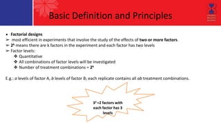
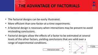
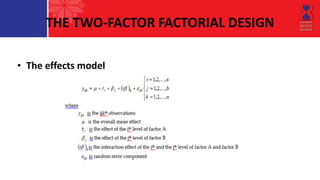
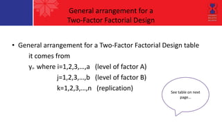
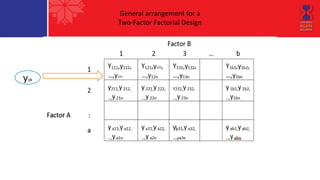
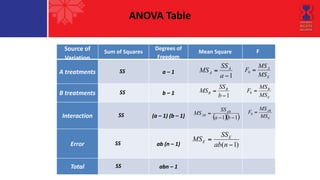
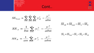
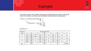
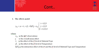
This document describes a two-factor factorial design experiment involving two factors, each with two levels. It defines what a factorial design is, how it is more efficient than single-factor experiments, and allows investigating interactions between factors. It provides an example of a 2x2 factorial design measuring the effects of two materials and two temperatures on battery life. Analysis of variance is performed on the example to investigate main effects and interactions between the factors.

1. TWO-­‐FACTOR
FACTORIAL
DESIGN
PREPARED
BY:
SITI
AISYAH
BT
NAWAWI

2. Basic
Definition
and
Principles
▪ Factorial
designs
➢
most
efficient
in
experiments
that
involve
the
study
of
the
effects
of
two
or
more
factors.
➢2k
means
there
are
k
factors
in
the
experiment
and
each
factor
has
two
levels
➢Factor
levels:
❖ Quantitative
❖ All
combinations
of
factor
levels
will
be
investigated
❖ Number
of
treatment
combinations
=
2k
!
E.g.:
a
levels
of
factor
A,
b
levels
of
factor
B;
each
replicate
contains
all
ab
treatment
combinations.
!!!!!!!!!
!!!
32
=2
factors
with
each
factor
has
3
levels

3. THE
ADVANTAGE
OF
FACTORIALS
!
• The
factorial
designs
can
be
easily
illustrated.
• More
efficient
than
one-­‐factor-­‐at-­‐a-­‐time
experiments.
• A
factorial
design
is
necessary
when
interactions
may
be
present
to
avoid
misleading
conclusions.
• Factorial
designs
allow
the
effects
of
a
factor
to
be
estimated
at
several
levels
of
the
other
factors,
yielding
conclusions
that
are
valid
over
a
range
of
experimental
conditions.
35
26
18
9
0
no alch. one alch
no barb.
one barb.
Interaction
exist

4. THE
TWO-­‐FACTOR
FACTORIAL
DESIGN
!
• The
effects
model

5. General
arrangement
for
a
Two-­‐Factor
Factorial
Design
!
• General
arrangement
for
a
Two-­‐Factor
Factorial
Design
table
it
comes
from
yijk
where
i=1,2,3,…,a
(level
of
factor
A)
j=1,2,3,…,b
(level
of
factor
B)
k=1,2,3,…,n
(replication) See
table
on
next
page…

6. General
arrangement
for
a
Two-­‐Factor
Factorial
Design
!
!
!
yijk

7. ANOVA
Table
Source
of
Variation
Sum
of
Squares Degrees
of
Freedom
Mean
Square F
A
treatments SS a
–
1
B
treatments SS b
–
1
Interaction SS (a
–
1)
(b
–
1)
Error SS ab
(n
–
1)
Total SS abn
–
1
MS SSA
−1
=
a
A
A
E
F MS 0 =
MS
MS SSB
−1
=
b
B
B
E
F MS 0 =
MS
MS SSAB
=
a b
( −1)( −1)
AB
AB
MS
E
F MS 0 =
MS SSE
=
ab n
( −1)
E

8. Cont..
a
ΣΣΣ
− = =
= − ⋅⋅⋅
Total ijk abn
i
b
j
n
k
y
SS y
1 1 1
2
2
y
1 ⋅⋅⋅
abn
y
= Σ −
A i
bn
SS
a
i
2
1
2.
.
=
y
1 ⋅⋅⋅
abn
y
= Σ −
B j
an
SS
b
j
2
1
2
. .
=
AB total A B SS = SS − SS − SS
E Total A B AB SS = SS − SS − SS − SS

9. Example

10. Cont..

11. cont..
• 2)
ANOVA
Now,
calculate
ANOVA
table
using
formula
given
in
previous
slide

12. Cont..
Source
of
Variation Sum
of
Squares
Degrees
of
Freedom
Mean
Square F
Material
types 10683.72 2 5,341.86 7.91
Temperature 39118.72 2 19,559.36 28.97
Interaction
(Material*Temperature)
9613.78 4 2,403.44 3.56
Error 18230.75 27 675.21
Total 77646.97 35

13. cont..

14. Cont..
Do
you
get
the
same
answer?
If
YES,
lets
continue..

15. Cont..

18. !
• Conclusion
:
This
analysis
indicates
that
at
the
temperature
level
700F,
the
mean
battery
life
is
the
same
for
material
types
2
and
3