Process optimization technique

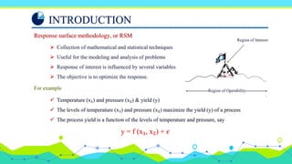
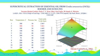
1. 1
RESPONSE SURFACE
METHODOLOGY (RSM)
Concept and its applications
M.Venkatasami, I.D.No: 2020641005
Ph.D. (Processing and Food Engineering)
Department of Food Process Engineering
AEC&RI, TNAU.

2. INTRODUCTION
Response surface methodology, or RSM
 Collection of mathematical and statistical techniques
 Useful for the modeling and analysis of problems
 Response of interest is influenced by several variables
 The objective is to optimize the response.
 Temperature (x₁) and pressure (x₂) & yield (y)
 The levels of temperature (x₁) and pressure (x₂) maximize the yield (y) of a process
 The process yield is a function of the levels of temperature and pressure, say
y = f (x₁, x₂) + 𝜖
For example
Region of Interest
Region of Operability

3. Run Temperature, C Pressure, bar
Total yield,
% dry basis
1 300 30 2.867
2 300 50 5.461
3 100 30 1.603
4 100 50 0.469
5 341 40 3.355
6 200 54 3.902
7 78 40 0.108
8 200 26 2.349
9 200 40 3.357
10 200 40 3.347
11 200 40 3.321
SUPERCRITICAL EXTRACTION OF ESSENTIAL OIL FROM Cordia curassavica (JACQ.)
ROEMER AND SCHULTES
(Quispe-Condori et al., 2003)
Socrates Quispe-Condori, Paulo T. V. Rosa, Mary Ann Foglio, M.Angela A. Meireles
LASEFI - DEA / FEA (College of Food Eng) – UNICAMP, Cx. P. 6121, 13083-970 Campinas, São Paulo, Brazil; 2CPQBA /
UNICAMP

4.  If we denote the expected response by E(y) = f (x₁, x₂) = 𝜂, then the surface represented by
 𝜂 = f (x₁, x₂)
 𝜂 = Response surface
 Contour plot: Contour corresponds to a particular
height of the response surface
CONT…
y = 𝛽₀ + 𝛽₁x₁ + 𝛽₂x₂ + · · · + 𝛽ₖxₖ + 𝜖
 If the response is well modeled by a linear function
of the independent variables, then the approximating
function is the first-order model
(Quispe-Condori et al., 2003)

5.  If there is curvature in the system, then a polynomial of higher degree must be used, such as
the second-order model
CONT…
𝒊−𝟏
𝒌
𝜷𝒊𝒙𝒊
𝒊−𝟏
𝒌
𝜷𝒊𝒊𝒙𝒊
𝟐
𝒊<𝒋
𝜷𝒊𝒋𝒊 𝒙𝒊𝒙𝒋
∑
+ + + ∈
+
y= 𝜷𝒐
 A relatively small region polynomial model usually work quite well
 The method of least squares is used to estimate the parameters in the polynomials.
 The response surface analysis is performed using the fitted surface
 The model parameters can be estimated most effectively if proper experimental designs are used
to collect the data.
 Designs for fitting response surfaces are called response surface designs.

6. CONT…
 RSM is a sequential procedure.
 The objective is to lead the experimenter
 A point on the response surface that is remote from the optimum
 Little curvature exist in the system
 The first-order model will be appropriate
 Rapidly and efficiently along a path of improvement
 Toward the general vicinity of the optimum.
 Once the region of the optimum has been found a more
elaborate model may be employed,
 The second-order model
 An analysis may be performed to locate the Optimum
(Montgomery 2017)

7. THE METHOD OF STEEPEST ASCENT
 A procedure for moving sequentially in the direction of the maximum increase in the response.
 If minimization is desired, then we call this technique the method of steepest descent.
 The fitted first-order model is,
𝑦 = 𝛽0+ ∑𝑖=1
𝑘
𝛽𝑖 𝑥𝑖
 In the first-order response surface,
 The contours of 𝑦 , is a series of parallel lines
 The direction of steepest ascent is the direction in which 𝑦
increases most rapidly.
 This direction is normal to the fitted response surface.
(Quispe-Condori et al., 2003)

8.  The path of steepest ascent ,
CONT…
 The steps along the path are proportional to the regression coefficients {𝛽0}.
 The actual step size is determined by the experimenter based on.
 Through the center of the region of interest
 Normal to the fitted surface
 Process knowledge
 Practical considerations
 The experimenter will arrive in the vicinity of the optimum
 New first-order model may be fit
 Indicated by lack of fit
Lack of fit
Significant Not significant

9. LOCATION OF THE STATIONARY POINT
 Suppose we wish to find the levels of x1, x2, . . . , xk that optimize the predicted response then x1,s, x2,s, .
. . , xk,s, is called the stationary point.
 The stationary point could represent a point of maximum response, a point of minimum response, or a
saddle point.

10. EXPERIMENTAL DESIGNS
 Fitting and analyzing response surfaces is greatly facilitated by the proper choice of an experimental
design
 The features of a desirable design are,
1. Provides a reasonable distribution of data
2. Allows model adequacy, including lack of fit, to be investigated
3. Allows experiments to be performed in blocks
4. Allows designs of higher order to be built up sequentially
5. Provides an internal estimate of error
6. Provides precise estimates of the model coefficients

11. 7. Provides a good profile of the prediction variance throughout the experimental region
8. Provides reasonable robustness against outliers or missing values
9. Does not require a large number of runs
10. Does not require too many levels of the independent variables
11. Ensures simplicity of calculation of the model parameters
CONT…
 Designs for Fitting the First-Order Model
𝒊−𝟏
𝒌
𝜷𝒊𝒙𝒊 + ∈
+
y= 𝜷𝒐
 A unique class of designs
 Minimize the variance of the regression coefficients {𝛽0}. .
 A first-order design is orthogonal
 The off-diagonal elements of the (X′X) matrix are all zero.
 This implies that the cross products of the columns of the x matrix sum to zero.

12. CONT…
 Designs includes the 2ᵏ factorial
 Fractions of the 2ᵏ series in which main effects are not aliased with each
other.
 The low and high levels of the k factors are coded to the usual ±1 levels.
 The 2ᵏ design does not afford an estimate of the experiments
 Replication - augment the design with several observations at the center
(the point xᵢ = 0, i = 1, 2, . . . , k).
 The addition of center points does not influence the {𝛽𝑖}. . for i ≥ 1, but
 The estimate of 𝛽₀ becomes the grand average of all observations.
 The addition of center points does not alter the orthogonality property of
the design
Run
Tempera
ture, C
Pressure
, bar
Total yield, % dry
basis
1 300 30 2.867
2 300 50 5.461
3 100 30 1.603
4 100 50 0.469
5 341 40 3.355
6 200 54 3.902
7 78 40 0.108
8 200 26 2.349
9 200 40 3.357
10 200 40 3.347
11 200 40 3.321
(Quispe-Condori et al., 2003)

13. CONT…
 Designs for Fitting the Second-Order Model
 The most popular class of designs used for fitting a second-order model is
the Central Composite Design or CCD
 The CCD consists of,
 A 2ᵏ factorial
 𝑛𝐹 Factorial runs
 2k axial or star runs
 𝑛𝐶Center runs
Central composite designs for k = 2(a) and k = 3(b)
 Practical deployment of a CCD
 Sequential experimentation

14. CONT…
 The distance 𝛼 of the axial runs from the design center
 The number of center points 𝑛𝐶
 Rotatability :  V(𝑦(𝑥)) − 𝑐𝑜𝑛𝑠𝑖𝑠𝑡𝑒𝑛𝑡 𝑎𝑛𝑑 𝑠𝑡𝑎𝑏𝑙𝑒  𝛼 = (𝑛𝐹)1/4
(Montgomery 2017)

15. CONT…
 The Box–Behnken Design
 Three-level designs (3ᵏ) for fitting response surfaces.
 These designs are formed by combining 2ᵏ factorials with
incomplete block designs.
 Very efficient in terms of the number of required runs
 Either rotatable or nearly rotatable.
 The experimental points are located at the center points of the
edges
 The centroid or center point of the experimental space is
replicated
Levels: -1,0,+1
3𝑘 k=3  27 Experiments
Three-level factorial.

16. Example 1

17. Example 2

18. REFERENCE
 Chohan, NA, G Aruwajoye, Y Sewsynker-Sukai, and EG Kana. 2020. "Valorisation of potato peel
wastes for bioethanol production using simultaneous saccharification and fermentation:
process optimization and kinetic assessment." Renewable Energy 146:1031-1040.
 Fisher, RA. 1936. "Design of experiments." Br Med J 1 (3923):554-554.
 Leardi, R. 2003. Design‐Expert 6.0, available from Stat‐Ease, Inc., 2021 E. Hennepin Avenue, Ste
480, Minneapolis, MN 55413‐2726, USA (E‐mail: info@ statease. com, Telephone:+
1‐612‐378‐9449, Fax:+ 1‐612‐378‐2152), Price: $995 for a single‐user licence. For further
information of current prices: http://www. statease. com/swprice. html. Wiley Online Library.

19.  Montgomery, DC. 2017. Design and analysis of experiments: John wiley & sons.
 Myers, RH, DC Montgomery, and CM Anderson-Cook. 2016. Response surface methodology: process and
product optimization using designed experiments: John Wiley & Sons.
 Pham, TM, W Sun, E Bujna, Á Hoschke, L Friedrich, and QD Nguyen. 2021. "Optimization of
Fermentation Conditions for Production of Hungarian Sour Cherry Spirit Using Response Surface
Methodology." Fermentation 7 (4):209.
 Quispe-Condori, S, PT Rosa, and MA Foglio. 2003. "Supercritical extraction of essential oil from Cordia
curassavica (Jacq.) Roemer and Schultes." Proceedings of the Sixth International Symposium on
Supercritical Fluids, Brunner, G., Kikic, I. and Perrut, M., Eds. ISASF, Versailles, France.
 Suliman, R. 2017. "Response Surface Methodology and Its Application in Optimizing the Efficiency of
Organic Solar Cells."
CONT…

20. THANK YOU