PRESENTATION ON
RESPONSE SURFACE METHODOLOGY
(RSM)
SUBJECT - OPTIMIZATION
BRANCH - CAD-CAM & ROBOTICS
PRESENTED BY
REGE PRATHAMESH MILIND (1605012)
TOPICS
INTRODUCTION TO RSM
LITERATURE REVIEW
WHEN DO WE USE RSM?
METHODOLOGY
EXAMPLE
APPLICATIONS
REFERENCES
INTRODUCTION TO RSM
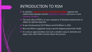
 In statistics, response surface methodology (RSM) explores the
relationships between several explanatory variables and one or more
response variables.
 The main idea of RSM is to use a sequence of designed experiments to
obtain an optimal response.
 It was introduced by G.E.P Wilson and K.B Wilson in 1951.
 Box and Wilson suggested using a second-degree polynomial model.
 It is only an approximation, but such a model is easy to estimate and
apply, even when little is known about the process.
CONTD.
Designed experiments with full
factorial design
Response surface with second-
degree polynomial
Source(http://LIONsolver.com/)
CONTD.
Main objectives are as follow.
1. Optimize.(main objective)
2. Develop.
3. Improve. (if necessary)
LITERATURE REVIEW
1. Xiaoyong Zhang, Jinyan Zhou, et al “Response surface methodology used for
statistical optimization of jiean-peptide production by Bacillus subtili,” Electronic
Journal of Biotechnology, Vol.13 No.4, Issue of July 15, 2010.
2. Kian Mun Lee and Sharifah Bee Abd Hamid,“Simple Response Surface
Methodology: Investigation on Advance Photocatalytic Oxidation of 4-
Chlorophenoxyacetic Acid Using UV-Active ZnO Photocatalyst,” Materials 2015, 8,
339-354; doi:10.3390/ma8010339
3. Russell V. Lenth,“Response-Surface Methods in R, Using rsm,” Journal of Statistical
Software, October 2009, Volume 32, Issue 7
WHEN DO WE USE RSM?
Source(http://LIONsolver.com/)
METHODOLOGY
 RSM resolve around the assumption that the response is a function of a
set of independent(design) variables x1,x2,x3….xk and function can be
approximated in some region of polynomial model.
𝑦=𝑓(𝑥_𝑖 )
𝑦=𝑓(𝑥_1,𝑥_2……𝑥_𝑘 )
Here response variable is “y” that depend on the “k” independent
variables.
 If the factors are given then directly estimate the effects and interaction of
model as describe in figure.
 And if the factors are unknown then first calculate them by using the
Screening method.
CONTD.
 Estimate The Interaction effect using 1st order model.
y = 𝛽0+𝛽1 𝑥1+𝛽2 𝑥2+𝜀
 If curvature is found then use the RSM. And 2nd order model will be used
to approximate the response variable.
 Make the graph and find the stationary point. Maximum response,
Minimum response or saddle point by using the obtained values of 𝑥_1,𝑥
_2,𝑥_3….𝑥_4.
TYPES OF MODELS
We use two types of model in RSM.
1. 1st Order Model.
2. 2nd Order Model.
WHEN TO USE WHICH MODEL?
 1STOrder Model.
Oftenly in RSM the relationship between response variable and Independent
variables is not given. After screening we use 1st order model to find current
situation and to find either there is curvature or not.
y = 𝛽_0+𝛽_1 𝑥_1+𝛽_2 𝑥_2+𝜀
 2nd Order Model
If we have find curvature after making fig from the result of 1st order model.
Then we use 2nd order model to find our optimum point.
Sequential Nature Of RSM.
Source(http://LIONsolver.com/)
METHODS OF RSM
 Steepest Ascent Method:
This is a procedure for moving sequentially in the direction of the
maximum increase in the response getting optimum response.
 Steepest Descent Method :
If minimization is desired then we call this technique the “method of
steepest descent”.
STEEPEST ASCENT METHOD
 This is a procedure for moving
sequentially in the direction of
the maximum increase in the
response getting optimum
response.
𝑦 = 𝛽𝑜 +
𝑖=1
𝑘
𝛽𝑖 𝑥𝑖
Source(http://LIONsolver.com/)
STEEPEST DESCENT METHOD
 If minimization is desired then we call
this technique the “method of
steepest descent”.
𝑦 = 𝛽𝑜 +
𝑖=1
𝑘
𝛽𝑖 𝑥𝑖
Source(http://LIONsolver.com/)
EXAMPLE
CONTD.
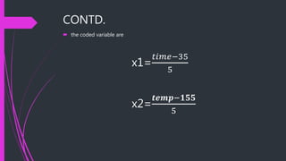
 the coded variable are
x1=
𝑡𝑖𝑚𝑒−35
5
x2=
𝒕𝒆𝒎𝒑−𝟏𝟓𝟓
5
CONTD.
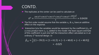
 The replicates at the center can be used to calculate an
𝜎2 =
(40.3)2+(40.5)2+ 40.7 2+ 40.2 2+ 40.6 2−
(202.3)2
5
4
= 0.0430
 The first order model assume that the variable 𝑥1 & 𝑥2 have an additive
effect on the response.
 Interaction b/w the variables would be represent by the coefficient 𝛽12 of
a cross product term 𝑥1 𝑥2 added to the model. the least square estimate
of this coefficient is just one half the interaction effect calculated as in an
ordinary 22
factorial design. Or
𝛽12 =
1
4
1 ∗ 39.3 + 1 ∗ 41.5 + −1 ∗ 40.0 + (−1 ∗ 40.9)
= -0.025
CONTD.
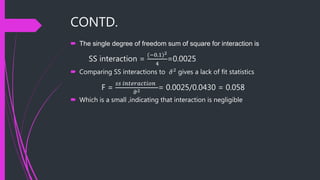
 The single degree of freedom sum of square for interaction is
SS interaction =
(−0.1)2
4
=0.0025
 Comparing SS interactions to 𝜎2 gives a lack of fit statistics
F =
𝑠𝑠 𝑖𝑛𝑡𝑒𝑟𝑎𝑐𝑡𝑖𝑜𝑛
𝜎2 = 0.0025/0.0430 = 0.058
 Which is a small ,indicating that interaction is negligible
APPLICATIONS
 The most frequent applications of RSM are in the industrial area.
 RSM is important in designing formulating and developing and analyzing
new specific scientific studying and product.
 It is also efficient in improvements of existing studies and products
 Most common application of RSM are in industrial ,biological and clinical
sciences, social sciences ,food sciences and physical and engineering
sciences
REFERENCES
1. Myers, R. H., and Montgomery, D. C., 1995, Response Surface Methodology, John
Wiley and Sons, Inc., New York, NY.
2. Bobillot, A. and Balmés, E. 2002, “Iterative Techniques for Eigenvalue Solutions of
Damped Structures Coupled with Fluids,” AIAA-2002-1391, American Institute of
Aeronautics and Astronautics.
3. Anderson, Mark J. and Whitcomb, Patrick J. 2004. “Design solutions from concept
through manufacture: Response surface methods for process optimization,” esktop
Engineering.(http://www.deskeng.com/)
THANK YOU

Resource Surface Methology

  • 1.
    PRESENTATION ON RESPONSE SURFACEMETHODOLOGY (RSM) SUBJECT - OPTIMIZATION BRANCH - CAD-CAM & ROBOTICS PRESENTED BY REGE PRATHAMESH MILIND (1605012)
  • 2.
    TOPICS INTRODUCTION TO RSM LITERATUREREVIEW WHEN DO WE USE RSM? METHODOLOGY EXAMPLE APPLICATIONS REFERENCES
  • 3.
    INTRODUCTION TO RSM In statistics, response surface methodology (RSM) explores the relationships between several explanatory variables and one or more response variables.  The main idea of RSM is to use a sequence of designed experiments to obtain an optimal response.  It was introduced by G.E.P Wilson and K.B Wilson in 1951.  Box and Wilson suggested using a second-degree polynomial model.  It is only an approximation, but such a model is easy to estimate and apply, even when little is known about the process.
  • 4.
    CONTD. Designed experiments withfull factorial design Response surface with second- degree polynomial Source(http://LIONsolver.com/)
  • 5.
    CONTD. Main objectives areas follow. 1. Optimize.(main objective) 2. Develop. 3. Improve. (if necessary)
  • 6.
    LITERATURE REVIEW 1. XiaoyongZhang, Jinyan Zhou, et al “Response surface methodology used for statistical optimization of jiean-peptide production by Bacillus subtili,” Electronic Journal of Biotechnology, Vol.13 No.4, Issue of July 15, 2010. 2. Kian Mun Lee and Sharifah Bee Abd Hamid,“Simple Response Surface Methodology: Investigation on Advance Photocatalytic Oxidation of 4- Chlorophenoxyacetic Acid Using UV-Active ZnO Photocatalyst,” Materials 2015, 8, 339-354; doi:10.3390/ma8010339 3. Russell V. Lenth,“Response-Surface Methods in R, Using rsm,” Journal of Statistical Software, October 2009, Volume 32, Issue 7
  • 7.
    WHEN DO WEUSE RSM? Source(http://LIONsolver.com/)
  • 8.
    METHODOLOGY  RSM resolvearound the assumption that the response is a function of a set of independent(design) variables x1,x2,x3….xk and function can be approximated in some region of polynomial model. 𝑦=𝑓(𝑥_𝑖 ) 𝑦=𝑓(𝑥_1,𝑥_2……𝑥_𝑘 ) Here response variable is “y” that depend on the “k” independent variables.  If the factors are given then directly estimate the effects and interaction of model as describe in figure.  And if the factors are unknown then first calculate them by using the Screening method.
  • 9.
    CONTD.  Estimate TheInteraction effect using 1st order model. y = 𝛽0+𝛽1 𝑥1+𝛽2 𝑥2+𝜀  If curvature is found then use the RSM. And 2nd order model will be used to approximate the response variable.  Make the graph and find the stationary point. Maximum response, Minimum response or saddle point by using the obtained values of 𝑥_1,𝑥 _2,𝑥_3….𝑥_4.
  • 10.
    TYPES OF MODELS Weuse two types of model in RSM. 1. 1st Order Model. 2. 2nd Order Model.
  • 11.
    WHEN TO USEWHICH MODEL?  1STOrder Model. Oftenly in RSM the relationship between response variable and Independent variables is not given. After screening we use 1st order model to find current situation and to find either there is curvature or not. y = 𝛽_0+𝛽_1 𝑥_1+𝛽_2 𝑥_2+𝜀  2nd Order Model If we have find curvature after making fig from the result of 1st order model. Then we use 2nd order model to find our optimum point.
  • 12.
    Sequential Nature OfRSM. Source(http://LIONsolver.com/)
  • 13.
    METHODS OF RSM Steepest Ascent Method: This is a procedure for moving sequentially in the direction of the maximum increase in the response getting optimum response.  Steepest Descent Method : If minimization is desired then we call this technique the “method of steepest descent”.
  • 14.
    STEEPEST ASCENT METHOD This is a procedure for moving sequentially in the direction of the maximum increase in the response getting optimum response. 𝑦 = 𝛽𝑜 + 𝑖=1 𝑘 𝛽𝑖 𝑥𝑖 Source(http://LIONsolver.com/)
  • 15.
    STEEPEST DESCENT METHOD If minimization is desired then we call this technique the “method of steepest descent”. 𝑦 = 𝛽𝑜 + 𝑖=1 𝑘 𝛽𝑖 𝑥𝑖 Source(http://LIONsolver.com/)
  • 16.
  • 17.
    CONTD.  the codedvariable are x1= 𝑡𝑖𝑚𝑒−35 5 x2= 𝒕𝒆𝒎𝒑−𝟏𝟓𝟓 5
  • 18.
    CONTD.  The replicatesat the center can be used to calculate an 𝜎2 = (40.3)2+(40.5)2+ 40.7 2+ 40.2 2+ 40.6 2− (202.3)2 5 4 = 0.0430  The first order model assume that the variable 𝑥1 & 𝑥2 have an additive effect on the response.  Interaction b/w the variables would be represent by the coefficient 𝛽12 of a cross product term 𝑥1 𝑥2 added to the model. the least square estimate of this coefficient is just one half the interaction effect calculated as in an ordinary 22 factorial design. Or 𝛽12 = 1 4 1 ∗ 39.3 + 1 ∗ 41.5 + −1 ∗ 40.0 + (−1 ∗ 40.9) = -0.025
  • 19.
    CONTD.  The singledegree of freedom sum of square for interaction is SS interaction = (−0.1)2 4 =0.0025  Comparing SS interactions to 𝜎2 gives a lack of fit statistics F = 𝑠𝑠 𝑖𝑛𝑡𝑒𝑟𝑎𝑐𝑡𝑖𝑜𝑛 𝜎2 = 0.0025/0.0430 = 0.058  Which is a small ,indicating that interaction is negligible
  • 20.
    APPLICATIONS  The mostfrequent applications of RSM are in the industrial area.  RSM is important in designing formulating and developing and analyzing new specific scientific studying and product.  It is also efficient in improvements of existing studies and products  Most common application of RSM are in industrial ,biological and clinical sciences, social sciences ,food sciences and physical and engineering sciences
  • 21.
    REFERENCES 1. Myers, R.H., and Montgomery, D. C., 1995, Response Surface Methodology, John Wiley and Sons, Inc., New York, NY. 2. Bobillot, A. and Balmés, E. 2002, “Iterative Techniques for Eigenvalue Solutions of Damped Structures Coupled with Fluids,” AIAA-2002-1391, American Institute of Aeronautics and Astronautics. 3. Anderson, Mark J. and Whitcomb, Patrick J. 2004. “Design solutions from concept through manufacture: Response surface methods for process optimization,” esktop Engineering.(http://www.deskeng.com/)
  • 22.