response

1. Internal Use
Response Surface Methodology – Part 2
Presented by
Gilford B. Estores, PhD

2. Internal Use
Topic Outline
1. 2K
Factorial Designs

3. Internal Use
2k
Factorial Designs
Factorial designs are frequently used in experiments involving several factors
where it is necessary to study the joint effect of the factors on a response.
However, several special cases of the general factorial design are important
because they are widely employed in research work and because they form the
basis of other designs of considerable practical value.
The most important of these special cases is that of k factors, each at only two
levels. These levels may be quantitative, such as two values of temperature,
pressure, or time; or they may be qualitative, such as two machines, two
operators, the “high’’ and “low’’ levels of a factor, or perhaps the presence and
absence of a factor. A complete replicate of such a design requires 2 x 2 x … x 2 =
2k
observations and is called a 2k
factorial design.

4. Internal Use
22
DESIGN
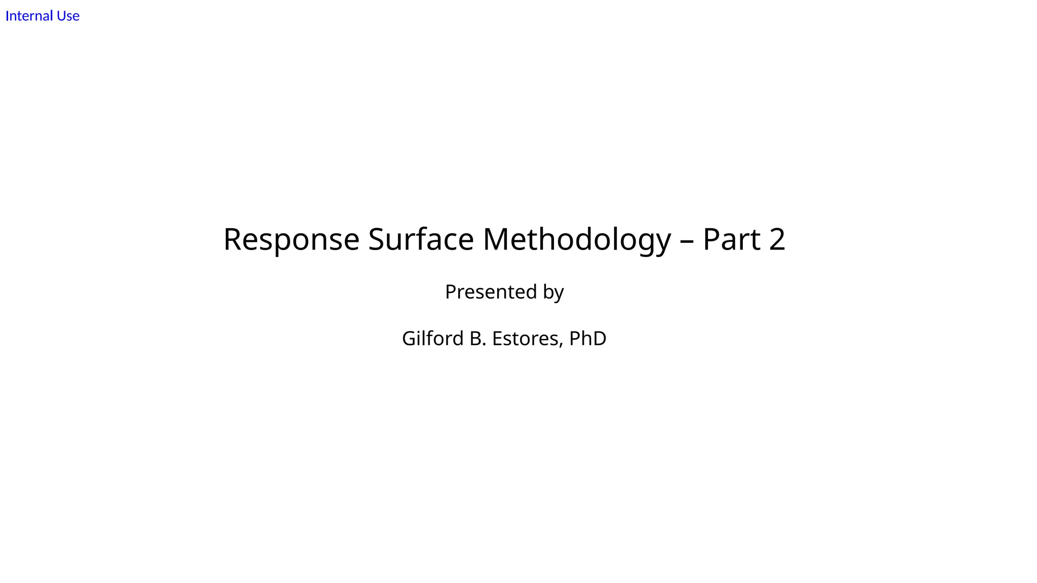
The simplest type of 2k
design is the 22
—that is, two factors A and B, each at two
levels. We usually think of these levels as the factor’s low and high levels.
In the 22
design, it is customary to denote the
low and high levels of the factors A and B by
the signs and +, respectively. This is
−
sometimes called the geometric notation for
the design.

5. Internal Use
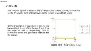
The main effect of B is found by averaging the observations on the top
of the square, where B is at the high level, and subtracting the
average of the observations on the bottom of the square, where B is
at the low level.
The main effect of A, we would average the observations on the right
side of the square in Fig. 14-15 where A is at the high level and subtract
from this the average of the observations on the left side of the square
where A is at the low level.

6. Internal Use
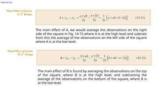
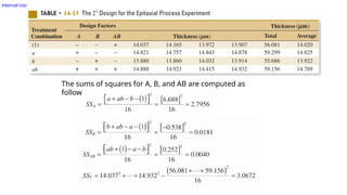
The AB interaction is estimated by taking the difference in the diagonal averages in Fig.
14-15. The quantities in brackets in Equations 14-11, 14-12, and 14-13 are called
contrasts. In these equations, the contrast coefficients are always either +1 or 1. A
−
table of plus and minus signs, such as Table 14-12, can be used to determine the sign on
each treatment combination for a particular contrast.
For example, the A contrast is
For example,

7. Internal Use
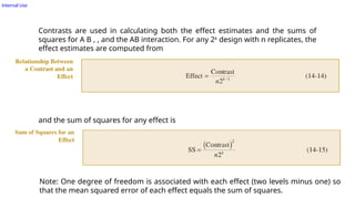
Contrasts are used in calculating both the effect estimates and the sums of
squares for A B , , and the AB interaction. For any 2k
design with n replicates, the
effect estimates are computed from
and the sum of squares for any effect is
Note: One degree of freedom is associated with each effect (two levels minus one) so
that the mean squared error of each effect equals the sum of squares.

8. Internal Use
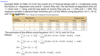
Example: Refer to Table 14-13 for the results of a 22
factorial design with n = 4 replicates using
the factors A = deposition time and B = arsenic flow rate. The two levels of deposition time are
= short and + = long, and the two levels of arsenic flow rate are = 55% and + = 59%. The
− −
response variable is epitaxial layer thickness (µm ) of the effects using Equations 14-11, 14-12,
and 14-13 as follows:
The estimates of the effects using Equations 14-11, 14-12, and 14-13 as
follows:

9. Internal Use
The sums of squares for A, B, and AB are computed as
follows:

10. Internal Use

11. Internal Use
2k
DESIGN FOR k 3 FACTORS
≥
The methods presented in the previous section for factorial designs with k=2
factors each at two levels can be easily extended to more than two factors. For
example, consider k=3 factors, each at two levels. This design is a 23
factorial
design, and it has eight runs or treatment combinations.
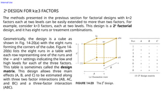
Geometrically, the design is a cube as
shown in Fig. 14-20(a) with the eight runs
forming the corners of the cube. Figure 14-
20(b) lists the eight runs in a table with
each row representing one of the runs and
the and + settings indicating the low and
−
high levels for each of the three factors.
This table is sometimes called the design
matrix. This design allows three main
effects (A, B, and C) to be estimated along
with three two factor interactions (AB, AC,
and BC) and a three-factor interaction
(ABC).

12. Internal Use
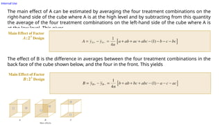
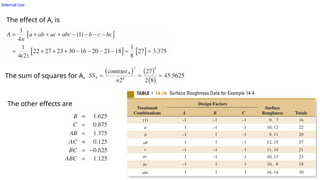
The main effect of A can be estimated by averaging the four treatment combinations on the
right-hand side of the cube where A is at the high level and by subtracting from this quantity
the average of the four treatment combinations on the left-hand side of the cube where A is
at the low level. This gives
The effect of B is the difference in averages between the four treatment combinations in the
back face of the cube shown below, and the four in the front. This yields

13. Internal Use
The effect of C is the difference in average response between the four treatment
combinations in the top face of the cube shown below and the four in the bottom, that is,
The two-factor interaction effects may be computed
easily. A measure of the AB interaction is the difference
between the average A effects at the two levels of B. By
convention, one-half of this difference is called the AB
interaction.

14. Internal Use
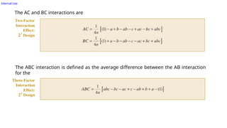
The AC and BC interactions are
The ABC interaction is defined as the average difference between the AB interaction
for the
two different levels of C.

15. Internal Use
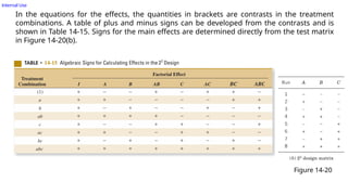
In the equations for the effects, the quantities in brackets are contrasts in the treatment
combinations. A table of plus and minus signs can be developed from the contrasts and is
shown in Table 14-15. Signs for the main effects are determined directly from the test matrix
in Figure 14-20(b).
Figure 14-20

16. Internal Use
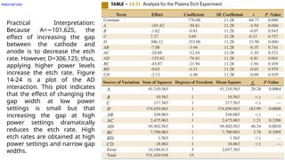
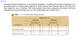
Example: Surface Roughness. A mechanical engineer is studying the surface roughness of a
part produced in a metal-cutting operation. Three factors, feed rate (A), depth of cut (B), and
tool angle (C), are of interest. All three factors have been assigned two levels, and two
replicates of a factorial design are run. The coded data are in Table 14-10.

17. Internal Use
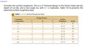
Consider the surface roughness. This is a 23
factorial design in the factors feed rate (A),
depth of cut (B), and a tool angle (C), with n = 2 replicates. Table 14-16 presents the
observed surface roughness data.

18. Internal Use
The effect of A, is
The sum of squares for A, is
The other effects are

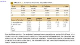
19. Internal Use
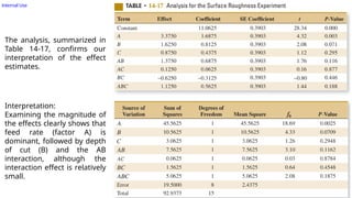
The analysis, summarized in
Table 14-17, confirms our
interpretation of the effect
estimates.
Interpretation:
Examining the magnitude of
the effects clearly shows that
feed rate (factor A) is
dominant, followed by depth
of cut (B) and the AB
interaction, although the
interaction effect is relatively
small.

20. Internal Use
SINGLE REPLICATE OF THE 2k
DESIGN
As the number of factors in a factorial experiment increases, the number of
effects that can be estimated also increases. For example, a 24
experiment
has 4 main effects, 6 two-factor interactions, 4 three-factor interactions, and 1
four-factor interaction, and a 26
experiment has 6 main effects, 15 two-factor
interactions, 20 three-factor interactions, 15 four-factor interactions, 6 five-
factor interactions, and 1 six-factor interaction.
In most situations, the sparsity of effects principle applies; that is, the system
is usually dominated by the main effects and low-order interactions. The
three-factor and higher order interactions are usually negligible.
Therefore, when the number of factors is moderately large, say, k 4 or 5, a
≥
common practice is to run only a single replicate of the 2k
design and then
pool or combine the higher order interactions as an estimate of error.
Sometimes a single replicate of a 2k
design is called an unreplicated 2k
factorial design.

21. Internal Use
Example 14-5: Plasma Etch. An article in Solid State Technology [“Orthogonal Design for
Process Optimization and Its Application in Plasma Etching” (May 1987, pp. 127–132)]
describes the application of factorial designs in developing a nitride etch process on a
single-wafer plasma etcher. The process uses C2 F6 as the reactant gas. It is possible to vary
the gas flow, the power applied to the cathode, the pressure in the reactor chamber, and
the spacing between the anode and the cathode (gap). Several response variables would
usually be of interest in this process, but in this example, we concentrate on etch rate for
silicon nitride.

22. Internal Use

23. Internal Use

24. Internal Use
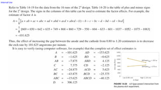
Practical Interpretation:
Because A= 101.625, the
−
effect of increasing the gap
between the cathode and
anode is to decrease the etch
rate. However, D=306.125; thus,
applying higher power levels
increase the etch rate. Figure
14-24 is a plot of the AD
interaction. This plot indicates
that the effect of changing the
gap width at low power
settings is small but that
increasing the gap at high
power settings dramatically
reduces the etch rate. High
etch rates are obtained at high
power settings and narrow gap
widths.

25. Internal Use
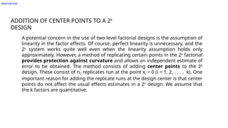
ADDITION OF CENTER POINTS TO A 2k
DESIGN
A potential concern in the use of two-level factorial designs is the assumption of
linearity in the factor effects. Of course, perfect linearity is unnecessary, and the
2k
system works quite well even when the linearity assumption holds only
approximately. However, a method of replicating certain points in the 2k
factorial
provides protection against curvature and allows an independent estimate of
error to be obtained. The method consists of adding center points to the 2k
design. These consist of nC replicates run at the point xi = 0 (i = 1, 2, . . . , k). One
important reason for adding the replicate runs at the design center is that center
points do not affect the usual effects estimates in a 2k
design. We assume that
the k factors are quantitative.

26. Internal Use
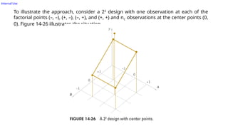
To illustrate the approach, consider a 22
design with one observation at each of the
factorial points (–, –), (+, –), (–, +), and (+, +) and nC observations at the center points (0,
0). Figure 14-26 illustrates the situation.

27. Internal Use
Let ȳF be the average of the four runs at the four factorial points and let yC be the average of
the nC run at the center point. If the difference ȳF - ȳC is small, the center points lie on or near
the plane passing through the factorial points, and there is no curvature. On the other hand,
if ȳF ȳ
− C is large, curvature is present.

28. Internal Use
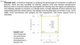
Example 14-6. A chemical engineer is studying the percentage of conversion or yield of a
process. There are two variables of interest, reaction time and reaction temperature.
Because she is uncertain about the assumption of linearity over the region of exploration,
the engineer decides to conduct a 22
design (with a single replicate of each factorial run)
augmented with five center points. The design and the yield data are shown in Fig. 14-27.
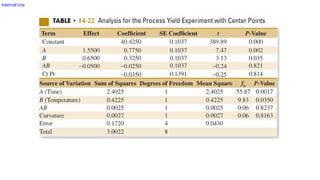
Table 14-22 summarizes the analysis for this experiment. The mean square error is
calculated from the center points as follows:

29. Internal Use

30. Internal Use
The mean square error is calculated from the center points

31. Internal Use
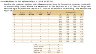
Problem Set No. 3 (Due on Nov. 4, 2024, 11:59 PM)
Considered a replicated two-level factorial experiment to study the factors most important to output in
an earth-moving system. Handle the experiment as four replicates of a 24
factorial design with
response equal to production rate (m3
/ h). The data are shown in the following table. Estimate the
factor effects and interpret.

32. Internal Use
Thank you for listening!