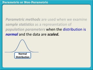
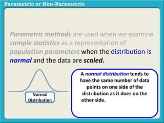
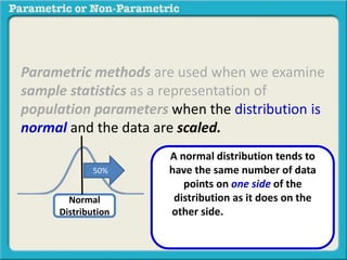
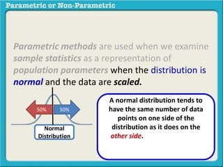
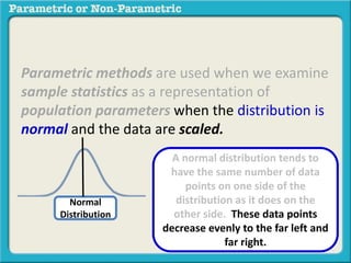
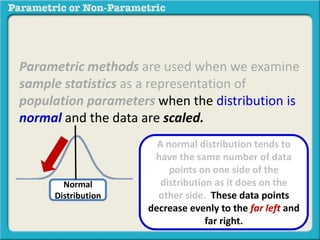
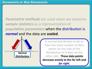
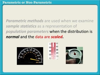
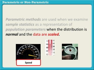
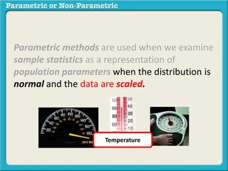
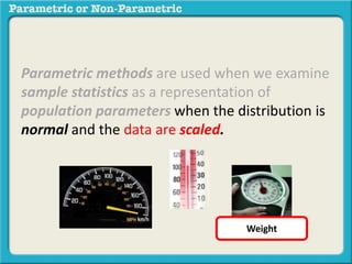
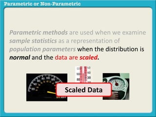
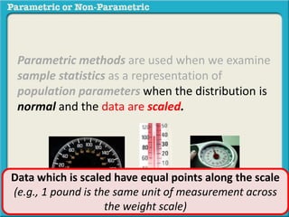
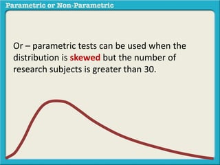
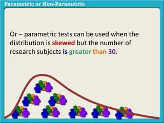
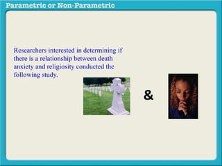
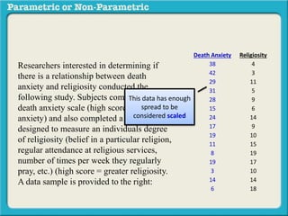
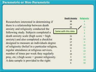
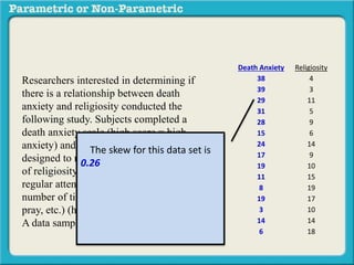
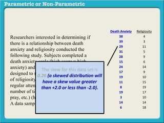
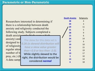
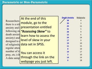
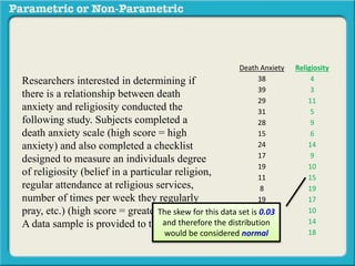
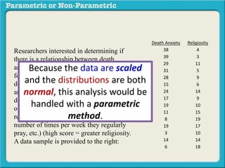
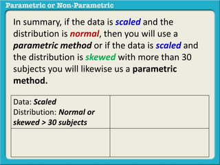
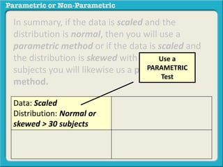
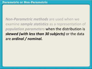
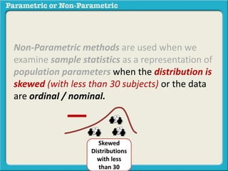
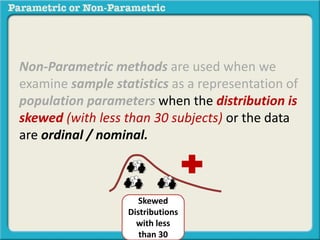
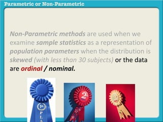
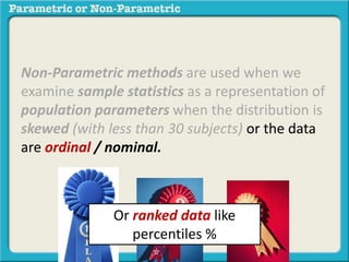
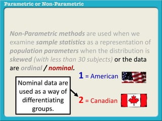
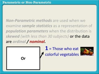
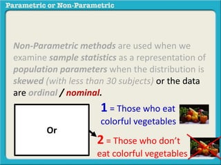
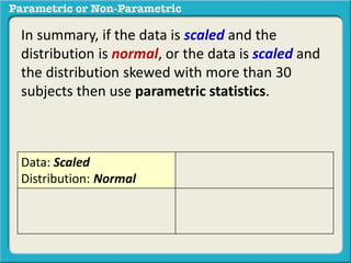
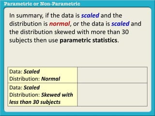
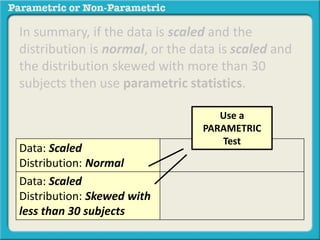
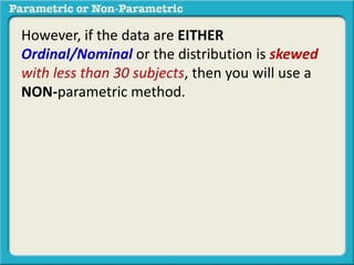
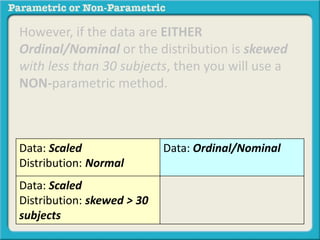
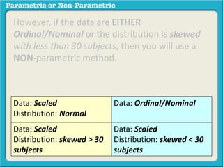
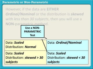
This presentation discusses parametric and non-parametric methods for analyzing relationships between variables. Parametric methods can be used when sample data is normally distributed and scaled, representing population parameters. They involve examining relationships between variables like death anxiety and religiosity through statistical tests. Non-parametric methods do not require normal distribution or scaling and can be used as an alternative.

1. Parametric or Nonparametric
Methods

2. This presentation is designed to help you
determine if using parametric or non-parametric
methods would be most appropriate with the
relationship question you are working on.

3. This presentation is designed to help you
determine if using parametric or non-parametric
methods would be most appropriate with the
relationship question you are working on.
Parametric Method
Non-Parametric Method

4. What are parametric methods?

5. Parametric methods are used when we examine
sample statistics

6. Parametric methods are used when we examine
sample statistics as a representation of
population parameters

7. Parametric methods are used when we examine
sample statistics as a representation of
population parameters when the distribution is
normal and the data are scaled.

8. Parametric methods are used when we examine
sample statistics as a representation of
population parameters when the distribution is
normal and the data are scaled.
Normal
Distribution

9. Parametric methods are used when we examine
sample statistics as a representation of
population parameters when the distribution is
normal and the data are scaled.
Normal
Distribution
A normal distribution tends to
have the same number of data
points on one side of the
distribution as it does on the
other side. These data points
decrease evenly to the far left and
far right.

10. Parametric methods are used when we examine
sample statistics as a representation of
population parameters when the distribution is
normal and the data are scaled.
Normal
Distribution
A normal distribution tends to
have the same number of data
points on one side of the
distribution as it does on the
other side. These data points
decrease evenly to the far left and
far right.
50%

11. Parametric methods are used when we examine
sample statistics as a representation of
population parameters when the distribution is
normal and the data are scaled.
Normal
Distribution
A normal distribution tends to
have the same number of data
points on one side of the
distribution as it does on the
other side. These data points
decrease evenly to the far left and
far right.
50%50%

12. Parametric methods are used when we examine
sample statistics as a representation of
population parameters when the distribution is
normal and the data are scaled.
Normal
Distribution
A normal distribution tends to
have the same number of data
points on one side of the
distribution as it does on the
other side. These data points
decrease evenly to the far left and
far right.

13. Parametric methods are used when we examine
sample statistics as a representation of
population parameters when the distribution is
normal and the data are scaled.
Normal
Distribution
A normal distribution tends to
have the same number of data
points on one side of the
distribution as it does on the
other side. These data points
decrease evenly to the far left and
far right.

14. Parametric methods are used when we examine
sample statistics as a representation of
population parameters when the distribution is
normal and the data are scaled.
Normal
Distribution
A normal distribution tends to
have the same number of data
points on one side of the
distribution as it does on the
other side. These data points
decrease evenly to the far left and
far right.

15. Parametric methods are used when we examine
sample statistics as a representation of
population parameters when the distribution is
normal and the data are scaled.

16. Parametric methods are used when we examine
sample statistics as a representation of
population parameters when the distribution is
normal and the data are scaled.
Speed

17. Parametric methods are used when we examine
sample statistics as a representation of
population parameters when the distribution is
normal and the data are scaled.
Temperature

18. Parametric methods are used when we examine
sample statistics as a representation of
population parameters when the distribution is
normal and the data are scaled.
Weight

19. Parametric methods are used when we examine
sample statistics as a representation of
population parameters when the distribution is
normal and the data are scaled.
Scaled Data

20. Parametric methods are used when we examine
sample statistics as a representation of
population parameters when the distribution is
normal and the data are scaled.
Data which is scaled have equal points along the scale
(e.g., 1 pound is the same unit of measurement across
the weight scale)

21. Or – parametric tests can be used when the
distribution is skewed but the number of
research subjects is greater than 30.

22. Or – parametric tests can be used when the
distribution is skewed but the number of
research subjects is greater than 30.

23. A parametric question that deals with
relationships might look like this:

24. Researchers interested in determining if
there is a relationship between death
anxiety and religiosity conducted the
following study. Subjects completed a
death anxiety scale (high score = high
anxiety) and also completed a checklist
designed to measure an individuals degree
of religiosity (belief in a particular religion,
regular attendance at religious services,
number of times per week they regularly
pray, etc.) (high score = greater religiosity.
A data sample is provided to the right:

25. Researchers interested in determining if
there is a relationship between death
anxiety and religiosity conducted the
following study. Subjects completed a
death anxiety scale (high score = high
anxiety) and also completed a checklist
designed to measure an individuals degree
of religiosity (belief in a particular religion,
regular attendance at religious services,
number of times per week they regularly
pray, etc.) (high score = greater religiosity.
A data sample is provided to the right:
&

26. Researchers interested in determining if
there is a relationship between death
anxiety and religiosity conducted the
following study. Subjects completed a
death anxiety scale (high score = high
anxiety) and also completed a checklist
designed to measure an individuals degree
of religiosity (belief in a particular religion,
regular attendance at religious services,
number of times per week they regularly
pray, etc.) (high score = greater religiosity.
A data sample is provided to the right:

27. Researchers interested in determining if
there is a relationship between death
anxiety and religiosity conducted the
following study. Subjects completed a
death anxiety scale (high score = high
anxiety) and also completed a checklist
designed to measure an individuals degree
of religiosity (belief in a particular religion,
regular attendance at religious services,
number of times per week they regularly
pray, etc.) (high score = greater religiosity.
A data sample is provided to the right:
Death Anxiety
Scale

28. Researchers interested in determining if
there is a relationship between death
anxiety and religiosity conducted the
following study. Subjects completed a
death anxiety scale (high score = high
anxiety) and also completed a checklist
designed to measure an individuals degree
of religiosity (belief in a particular religion,
regular attendance at religious services,
number of times per week they regularly
pray, etc.) (high score = greater religiosity.
A data sample is provided to the right:

29. Researchers interested in determining if
there is a relationship between death
anxiety and religiosity conducted the
following study. Subjects completed a
death anxiety scale (high score = high
anxiety) and also completed a checklist
designed to measure an individuals degree
of religiosity (belief in a particular religion,
regular attendance at religious services,
number of times per week they regularly
pray, etc.) (high score = greater religiosity.)
A data sample is provided to the right:

30. Researchers interested in determining if
there is a relationship between death
anxiety and religiosity conducted the
following study. Subjects completed a
death anxiety scale (high score = high
anxiety) and also completed a checklist
designed to measure an individuals degree
of religiosity (belief in a particular religion,
regular attendance at religious services,
number of times per week they regularly
pray, etc.) (high score = greater religiosity.)
A data sample is provided to the right:

31. Researchers interested in determining if
there is a relationship between death
anxiety and religiosity conducted the
following study. Subjects completed a
death anxiety scale (high score = high
anxiety) and also completed a checklist
designed to measure an individuals degree
of religiosity (belief in a particular religion,
regular attendance at religious services,
number of times per week they regularly
pray, etc.) (high score = greater religiosity).
A data sample is provided to the right:
Measure of
Religiosity

32. Researchers interested in determining if
there is a relationship between death
anxiety and religiosity conducted the
following study. Subjects completed a
death anxiety scale (high score = high
anxiety) and also completed a checklist
designed to measure an individuals degree
of religiosity (belief in a particular religion,
regular attendance at religious services,
number of times per week they regularly
pray, etc.) (high score = greater religiosity.
A data sample is provided to the right:

33. Death Anxiety Religiosity
38 4
42 3
29 11
31 5
28 9
15 6
24 14
17 9
19 10
11 15
8 19
19 17
3 10
14 14
6 18
Researchers interested in determining if
there is a relationship between death
anxiety and religiosity conducted the
following study. Subjects completed a
death anxiety scale (high score = high
anxiety) and also completed a checklist
designed to measure an individuals degree
of religiosity (belief in a particular religion,
regular attendance at religious services,
number of times per week they regularly
pray, etc.) (high score = greater religiosity.
A data sample is provided to the right:

34. Death Anxiety Religiosity
38 4
42 3
29 11
31 5
28 9
15 6
24 14
17 9
19 10
11 15
8 19
19 17
3 10
14 14
6 18
Researchers interested in determining if
there is a relationship between death
anxiety and religiosity conducted the
following study. Subjects completed a
death anxiety scale (high score = high
anxiety) and also completed a checklist
designed to measure an individuals degree
of religiosity (belief in a particular religion,
regular attendance at religious services,
number of times per week they regularly
pray, etc.) (high score = greater religiosity.
A data sample is provided to the right:
This data has enough
spread to be
considered scaled

35. Death Anxiety Religiosity
38 4
39 3
29 11
31 5
28 9
15 6
24 14
17 9
19 10
11 15
8 19
19 17
3 10
14 14
6 18
Researchers interested in determining if
there is a relationship between death
anxiety and religiosity conducted the
following study. Subjects completed a
death anxiety scale (high score = high
anxiety) and also completed a checklist
designed to measure an individuals degree
of religiosity (belief in a particular religion,
regular attendance at religious services,
number of times per week they regularly
pray, etc.) (high score = greater religiosity.
A data sample is provided to the right:
Same with this data.

36. Death Anxiety Religiosity
38 4
39 3
29 11
31 5
28 9
15 6
24 14
17 9
19 10
11 15
8 19
19 17
3 10
14 14
6 18
Researchers interested in determining if
there is a relationship between death
anxiety and religiosity conducted the
following study. Subjects completed a
death anxiety scale (high score = high
anxiety) and also completed a checklist
designed to measure an individuals degree
of religiosity (belief in a particular religion,
regular attendance at religious services,
number of times per week they regularly
pray, etc.) (high score = greater religiosity.
A data sample is provided to the right:
The skew for this data set is
0.26 (a skewed distribution will
have a skew value greater
than +2.0 or less than -2.0).
While slightly skewed to the
right, the distribution would be
considered normal

37. Death Anxiety Religiosity
38 4
39 3
29 11
31 5
28 9
15 6
24 14
17 9
19 10
11 15
8 19
19 17
3 10
14 14
6 18
Researchers interested in determining if
there is a relationship between death
anxiety and religiosity conducted the
following study. Subjects completed a
death anxiety scale (high score = high
anxiety) and also completed a checklist
designed to measure an individuals degree
of religiosity (belief in a particular religion,
regular attendance at religious services,
number of times per week they regularly
pray, etc.) (high score = greater religiosity.
A data sample is provided to the right:
The skew for this data set is
0.26 (a skewed distribution will
have a skew value greater
than +2.0 or less than -2.0).
While slightly skewed to the
right, the distribution would be
considered normal

38. Death Anxiety Religiosity
38 4
39 3
29 11
31 5
28 9
15 6
24 14
17 9
19 10
11 15
8 19
19 17
3 10
14 14
6 18
Researchers interested in determining if
there is a relationship between death
anxiety and religiosity conducted the
following study. Subjects completed a
death anxiety scale (high score = high
anxiety) and also completed a checklist
designed to measure an individuals degree
of religiosity (belief in a particular religion,
regular attendance at religious services,
number of times per week they regularly
pray, etc.) (high score = greater religiosity.
A data sample is provided to the right:
The skew for this data set is
0.26 (a skewed distribution will
have a skew value greater
than +2.0 or less than -2.0).
While slightly skewed to the
right, the distribution would be
considered normal

39. Death Anxiety Religiosity
38 4
39 3
29 11
31 5
28 9
15 6
24 14
17 9
19 10
11 15
8 19
19 17
3 10
14 14
6 18
Researchers interested in determining if
there is a relationship between death
anxiety and religiosity conducted the
following study. Subjects completed a
death anxiety scale (high score = high
anxiety) and also completed a checklist
designed to measure an individuals degree
of religiosity (belief in a particular religion,
regular attendance at religious services,
number of times per week they regularly
pray, etc.) (high score = greater religiosity.
A data sample is provided to the right:
At the end of this
module, go to the
presentation entitled
“Assessing Skew” to
learn how to assess the
level of skew in your
data set in SPSS.
You can access it
through the link on the
webpage you just left.

40. Death Anxiety Religiosity
38 4
39 3
29 11
31 5
28 9
15 6
24 14
17 9
19 10
11 15
8 19
19 17
3 10
14 14
6 18
Researchers interested in determining if
there is a relationship between death
anxiety and religiosity conducted the
following study. Subjects completed a
death anxiety scale (high score = high
anxiety) and also completed a checklist
designed to measure an individuals degree
of religiosity (belief in a particular religion,
regular attendance at religious services,
number of times per week they regularly
pray, etc.) (high score = greater religiosity.
A data sample is provided to the right:
The skew for this data set is 0.03
and therefore the distribution
would be considered normal

41. Death Anxiety Religiosity
38 4
39 3
29 11
31 5
28 9
15 6
24 14
17 9
19 10
11 15
8 19
19 17
3 10
14 14
6 18
Researchers interested in determining if
there is a relationship between death
anxiety and religiosity conducted the
following study. Subjects completed a
death anxiety scale (high score = high
anxiety) and also completed a checklist
designed to measure an individuals degree
of religiosity (belief in a particular religion,
regular attendance at religious services,
number of times per week they regularly
pray, etc.) (high score = greater religiosity.
A data sample is provided to the right:
Because the data are scaled
and the distributions are both
normal, this analysis would be
handled with a parametric
method.

42. In summary,

43. In summary, if the data is scaled and the
distribution is normal, then you will use a
parametric method or if the data is scaled and
the distribution is skewed with more than 30
subjects you will likewise us a parametric
method.

44. In summary, if the data is scaled and the
distribution is normal, then you will use a
parametric method or if the data is scaled and
the distribution is skewed with more than 30
subjects you will likewise us a parametric
method.
Data: Scaled
Distribution: Normal or
skewed > 30 subjects

45. In summary, if the data is scaled and the
distribution is normal, then you will use a
parametric method or if the data is scaled and
the distribution is skewed with more than 30
subjects you will likewise us a parametric
method.
Data: Scaled
Distribution: Normal or
skewed > 30 subjects
Use a
PARAMETRIC
Test

46. What are nonparametric methods?

47. Non-Parametric methods are used when we
examine sample statistics

48. Non-Parametric methods are used when we
examine sample statistics as a representation of
population parameters

49. Non-Parametric methods are used when we
examine sample statistics as a representation of
population parameters when the distribution is
skewed (with less than 30 subjects) or the data
are ordinal / nominal.

50. Non-Parametric methods are used when we
examine sample statistics as a representation of
population parameters when the distribution is
skewed (with less than 30 subjects) or the data
are ordinal / nominal.
Skewed
Distributions
with less
than 30

51. Non-Parametric methods are used when we
examine sample statistics as a representation of
population parameters when the distribution is
skewed (with less than 30 subjects) or the data
are ordinal / nominal.
Skewed
Distributions
with less
than 30

52. Non-Parametric methods are used when we
examine sample statistics as a representation of
population parameters when the distribution is
skewed (with less than 30 subjects) or the data
are ordinal / nominal.

53. Non-Parametric methods are used when we
examine sample statistics as a representation of
population parameters when the distribution is
skewed (with less than 30 subjects) or the data
are ordinal / nominal.
Or ranked data like
percentiles %

54. Non-Parametric methods are used when we
examine sample statistics as a representation of
population parameters when the distribution is
skewed (with less than 30 subjects) or the data
are ordinal / nominal.

55. Non-Parametric methods are used when we
examine sample statistics as a representation of
population parameters when the distribution is
skewed (with less than 30 subjects) or the data
are ordinal / nominal.
1 = American
2 = Canadian

56. Non-Parametric methods are used when we
examine sample statistics as a representation of
population parameters when the distribution is
skewed (with less than 30 subjects) or the data
are ordinal / nominal.
1 = American
2 = Canadian
Nominal data are
used as a way of
differentiating
groups.

57. Non-Parametric methods are used when we
examine sample statistics as a representation of
population parameters when the distribution is
skewed (with less than 30 subjects) or the data
are ordinal / nominal.
1 = American
2 = Canadian
Nominal data are
used as a way of
differentiating
groups.

58. Non-Parametric methods are used when we
examine sample statistics as a representation of
population parameters when the distribution is
skewed (with less than 30 subjects) or the data
are ordinal / nominal.
1 = American
2 = Canadian
Nominal data are
used as a way of
differentiating
groups.

59. Non-Parametric methods are used when we
examine sample statistics as a representation of
population parameters when the distribution is
skewed (with less than 30 subjects) or the data
are ordinal / nominal.
Or
1 = Those who eat
colorful vegetables

60. Non-Parametric methods are used when we
examine sample statistics as a representation of
population parameters when the distribution is
skewed (with less than 30 subjects) or the data
are ordinal / nominal.
Or
1 = Those who eat
colorful vegetables
2 = Those who don’t
eat colorful vegetables

61. A nonparametric question that deals with
relationships might look like this:

62. Determine whether the following Beatle’s album top 40
rankings is related to the albums’ sales-rankings from
1965 to 1970.

63. Determine whether the following Beatle’s album top 40
rankings is related to the albums’ sales-rankings from
1965 to 1970.
Album Year
Top 40
Rank
Sales
Rank
Beatles for Sale 1965 1 1
Rubber Soul 1965 2 1
Revolver 1966 3 3
Sgt. Pepper 1967 1 2
Magical Mystery Tour 1967 3 4
The Beatles (white album) 1968 6 2
Abbey Road 1969 7 3
Let it Be 1970 4 5
Album Top 40 & Sales Rank

64. Determine whether the following Beatle’s album top 40
rankings is related to the albums’ sales-rankings from
1965 to 1970.
Album Year
Top 40
Rank
Sales
Rank
Beatles for Sale 1965 1 1
Rubber Soul 1965 2 1
Revolver 1966 3 3
Sgt. Pepper 1967 1 2
Magical Mystery Tour 1967 3 4
The Beatles (white album) 1968 6 2
Abbey Road 1969 7 3
Let it Be 1970 4 5
Album Top 40 & Sales Rank
Both sets of data
are ordinal or rank
ordered

65. Determine whether the following Beatle’s album top 40
rankings is related to the albums’ sales-rankings from
1965 to 1970.
Album Year
Top 40
Rank
Sales
Rank
Beatles for Sale 1965 1 1
Rubber Soul 1965 2 1
Revolver 1966 3 3
Sgt. Pepper 1967 1 2
Magical Mystery Tour 1967 3 4
The Beatles (white album) 1968 6 2
Abbey Road 1969 7 3
Let it Be 1970 4 5
Album Top 40 & Sales Rank
Both sets of data
are ordinal or rank
ordered

66. Determine whether the following Beatle’s album top 40
rankings is related to the albums’ sales-rankings from
1965 to 1970.
Because the data are ordinal
this analysis would be handled
with a nonparametric method.

67. Very Important Note –
When the data are ordinal in at least
ONE data set we will automatically use
a nonparametric test, regardless of
whether the distribution is normal or
not.regardless of whether the
distribution is normal or not.

68. Very Important Note –
When the data are ordinal in at least
ONE data set we will automatically use
a nonparametric test, regardless of
whether the distribution is normal or
not.regardless of whether the
distribution is normal or not.

69. Very Important Note –
When the data are ordinal in at least
ONE data set we will automatically use
a nonparametric test, regardless of
whether the distribution is normal or
not.

70. Here is another nonparametric-relationship
problem:

71. Do those from rural areas tend to drink more
than 8 ounces of an alcoholic beverage in one
sitting than those from urban areas?

72. Do those from rural areas tend to drink more
than 8 ounces of an alcoholic beverage in one
sitting than those from urban areas?
Where the subject
is from?
Amount of
alcohol drunken
Subject
Rural = 1
City = 2
Less than 8oz = 1
More than 8oz = 2
a 1 1
b 1 1
c 1 2
d 1 1
e 2 2
f 2 1
g 2 1
h 2 1

73. Do those from rural areas tend to drink more
than 8 ounces of an alcoholic beverage in one
sitting than those from urban areas?
Where the subject
is from?
Amount of
alcohol drunken
Subject
Rural = 1
City = 2
Less than 8oz = 1
More than 8oz = 2
a 1 1
b 1 1
c 1 2
d 1 1
e 2 2
f 2 1
g 2 1
h 2 1
Both sets of
data are
nominal
(either/or)

74. Do those from rural areas tend to drink more
than 8 ounces of an alcoholic beverage in one
sitting than those from urban areas?
Where the subject
is from?
Amount of
alcohol drunken
Subject
Rural = 1
City = 2
Less than 8oz = 1
More than 8oz = 2
a 1 1
b 1 1
c 1 2
d 1 1
e 2 2
f 2 1
g 2 1
h 2 1
Both sets of
data are
nominal
(either/or)
Because the data are nominal
this analysis would be handled
with a nonparametric method.

75. The Same Very Important Note –
When the data are nominal in at least
ONE data set we will automatically use
a nonparametric test, regardless of
whether the distribution is normal or
not.regardless of whether the
distribution is normal or not.

76. The Same Very Important Note –
When the data are nominal in at least
ONE data set we will automatically use
a nonparametric test, regardless of
whether the distribution is normal or
not.regardless of whether the
distribution is normal or not.

77. The Same Very Important Note –
When the data are nominal in at least
ONE data set we will automatically use
a nonparametric test, regardless of
whether the distribution is normal or
not.

78. In summary,

79. In summary, if the data is scaled and the
distribution is normal, or the data is scaled and
the distribution skewed with more than 30
subjects then use parametric statistics.

80. In summary, if the data is scaled and the
distribution is normal, or the data is scaled and
the distribution skewed with more than 30
subjects then use parametric statistics.
Data: Scaled
Distribution: Normal

81. In summary, if the data is scaled and the
distribution is normal, or the data is scaled and
the distribution skewed with more than 30
subjects then use parametric statistics.
Data: Scaled
Distribution: Normal
Data: Scaled
Distribution: Skewed with
less than 30 subjects

82. In summary, if the data is scaled and the
distribution is normal, or the data is scaled and
the distribution skewed with more than 30
subjects then use parametric statistics.
Data: Scaled
Distribution: Normal
Data: Scaled
Distribution: Skewed with
less than 30 subjects
Use a
PARAMETRIC
Test

83. However, if the data are EITHER
Ordinal/Nominal or the distribution is skewed
with less than 30 subjects, then you will use a
NON-parametric method.

84. However, if the data are EITHER
Ordinal/Nominal or the distribution is skewed
with less than 30 subjects, then you will use a
NON-parametric method.
Data: Scaled
Distribution: Normal
Data: Ordinal/Nominal
Data: Scaled
Distribution: skewed > 30
subjects

85. However, if the data are EITHER
Ordinal/Nominal or the distribution is skewed
with less than 30 subjects, then you will use a
NON-parametric method.
Data: Scaled
Distribution: Normal
Data: Ordinal/Nominal
Data: Scaled
Distribution: skewed > 30
subjects
Data: Scaled
Distribution: skewed < 30
subjects

86. However, if the data are EITHER
Ordinal/Nominal or the distribution is skewed
with less than 30 subjects, then you will use a
NON-parametric method.
Data: Scaled
Distribution: Normal
Data: Ordinal/Nominal
Data: Scaled
Distribution: skewed > 30
subjects
Data: Scaled
Distribution: skewed < 30
subjects
Use a NON-
PARAMETRIC
Test

87. What type of method would be most
appropriate for the data set you are
working with?

88. What type of method would be most
appropriate for the data set you are
working with?
Parametric Method
Non-Parametric Method