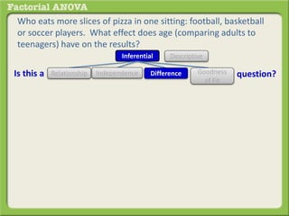
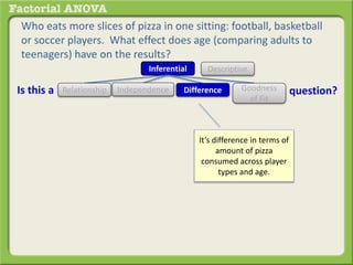
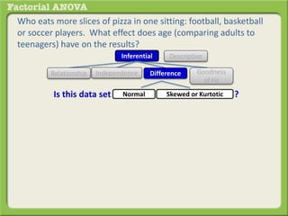
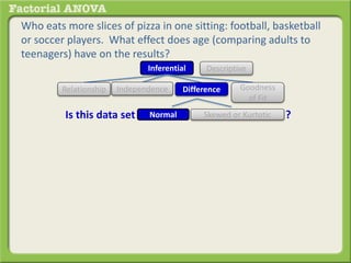
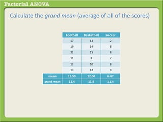
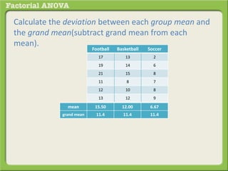
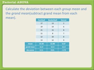
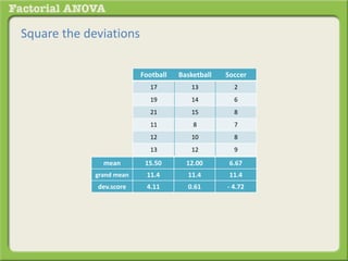
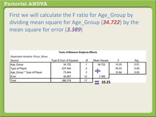
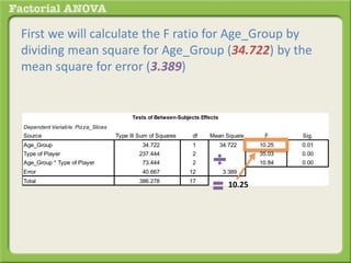
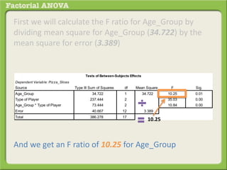
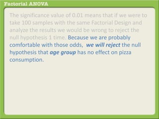
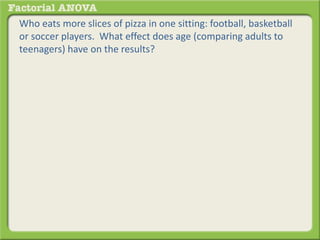
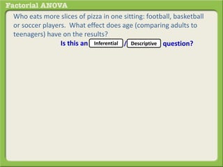
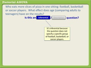
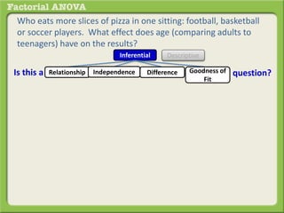
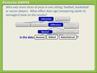
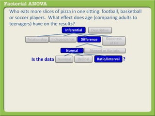
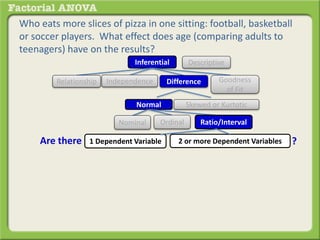
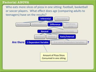
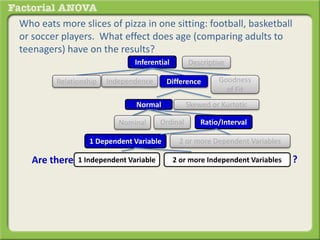
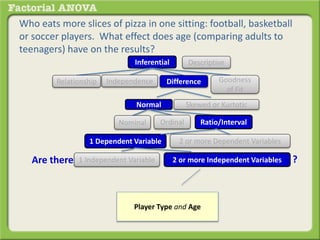
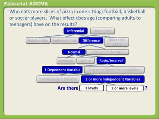
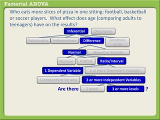
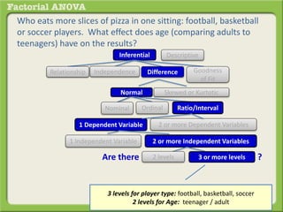
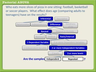
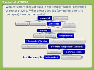
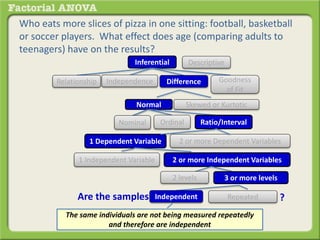
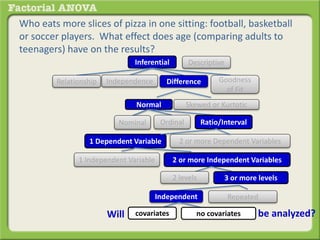
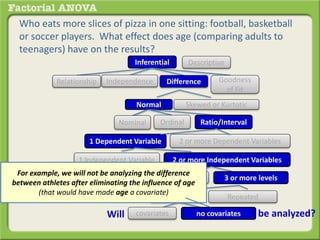
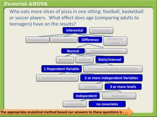
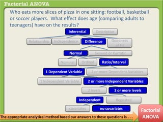
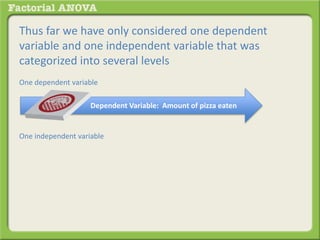
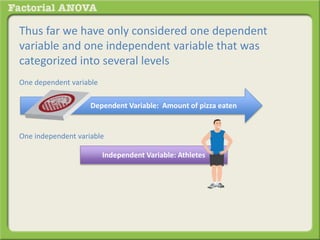
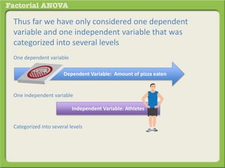
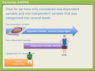
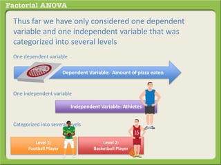
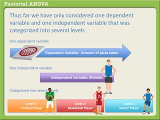
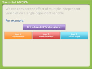
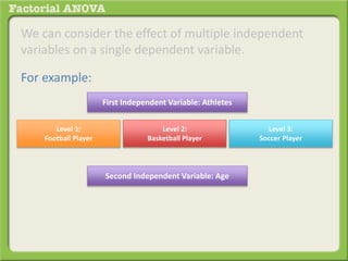
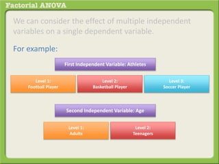
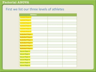
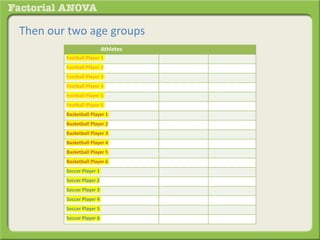
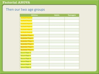
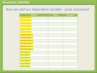
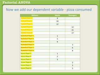
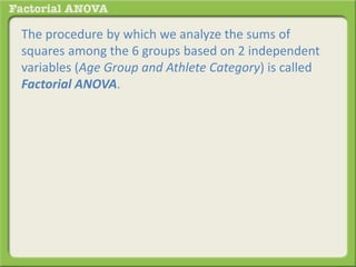
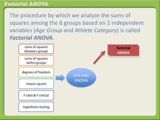
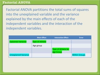
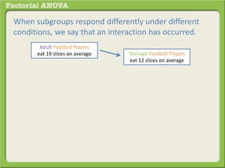
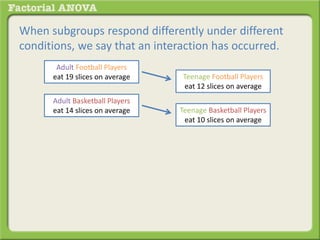
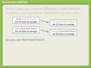
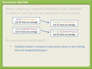
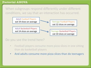
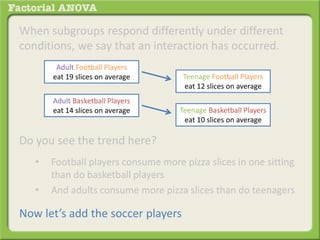
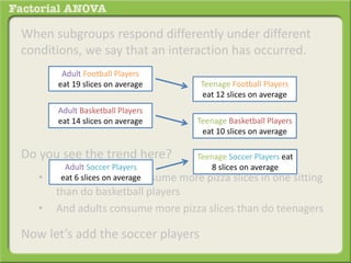
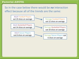
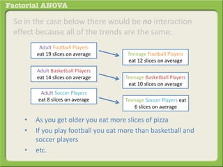
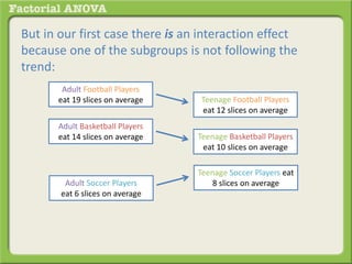
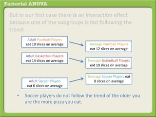
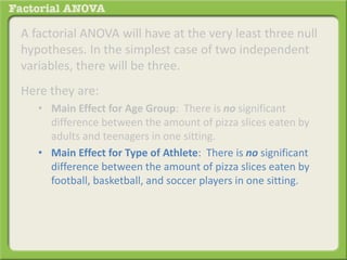
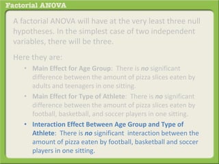
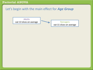
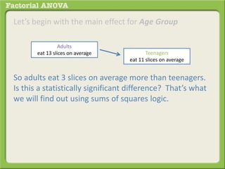
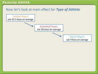
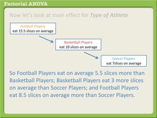
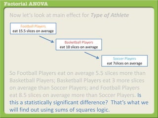
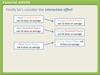
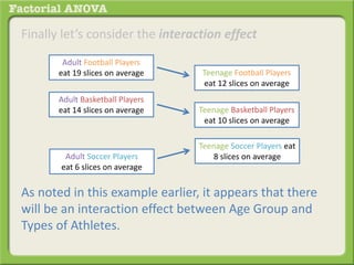
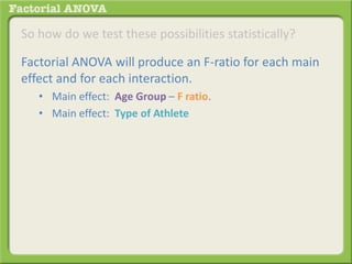
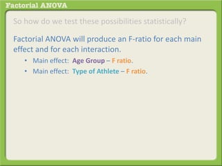
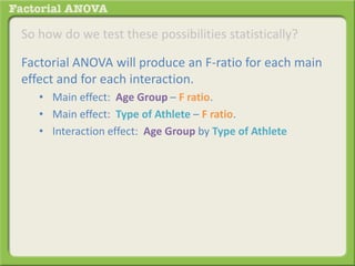
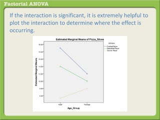
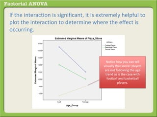
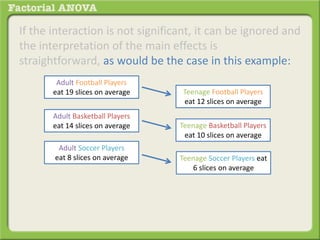
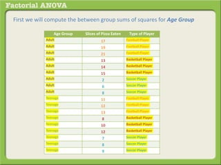
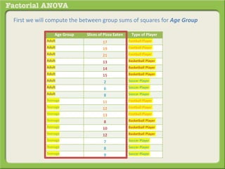
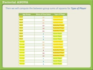
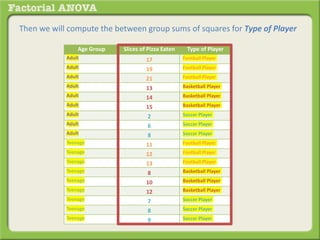
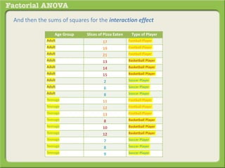
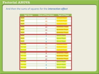
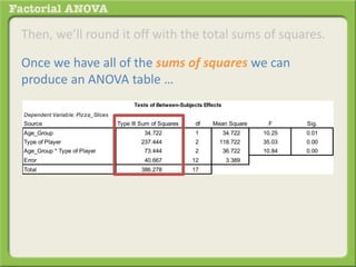
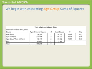
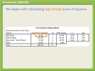
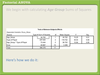
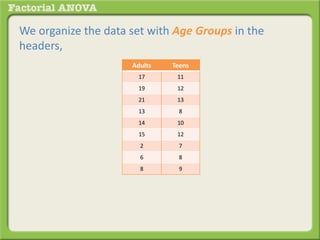
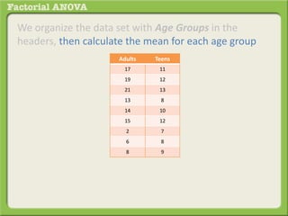
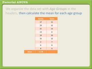
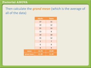
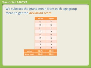
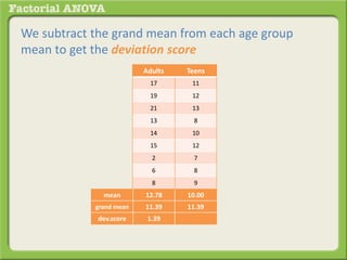
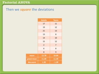
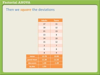
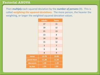
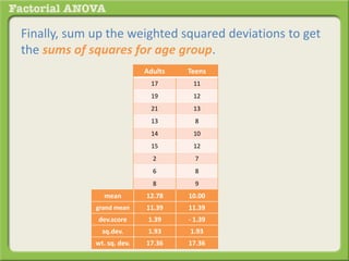
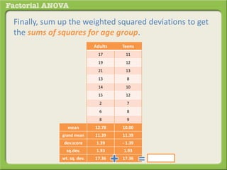
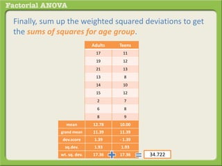
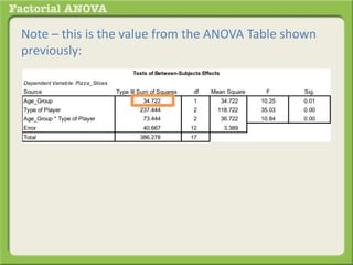
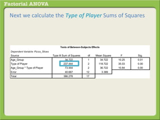
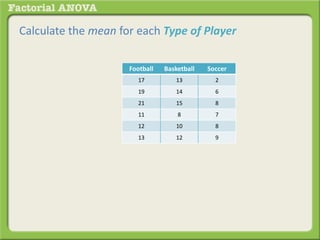
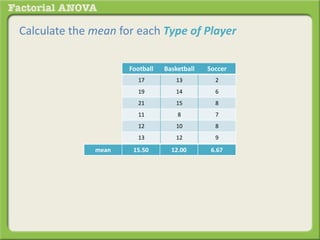
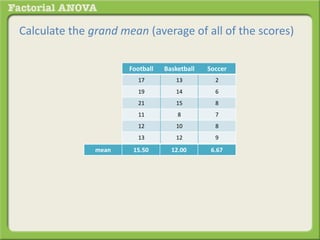
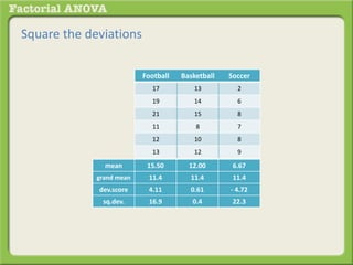
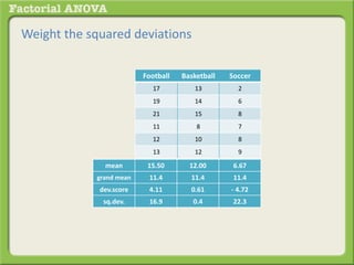
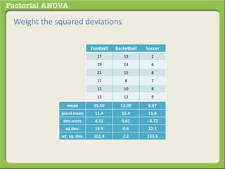
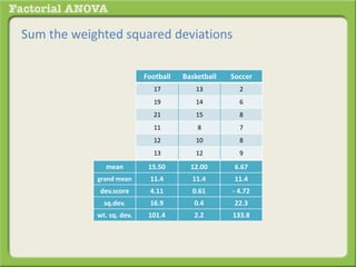
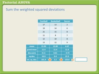
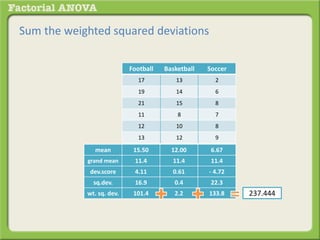
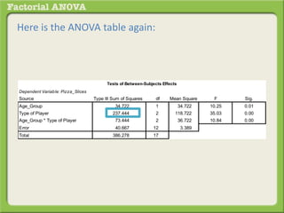
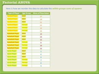
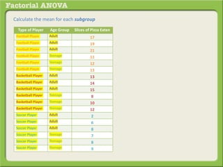
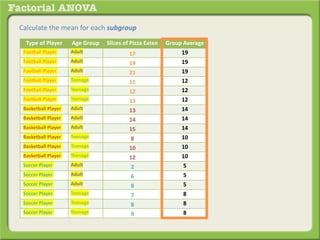
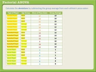
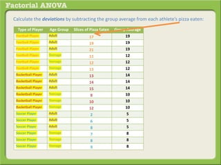
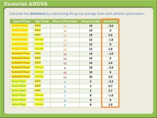
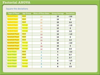
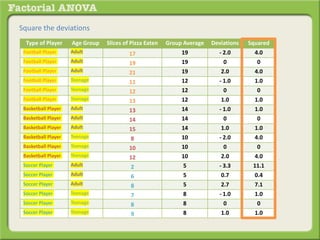
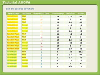
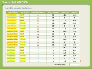
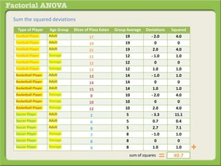
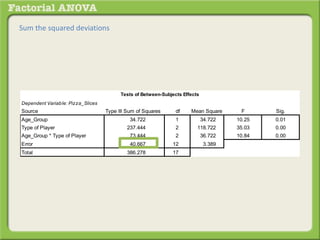
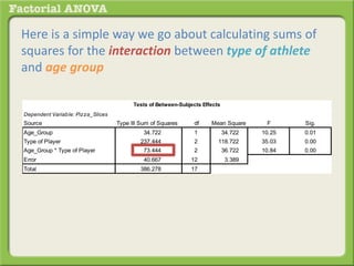
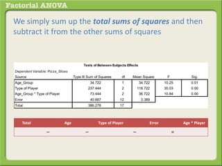
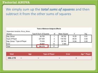
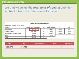
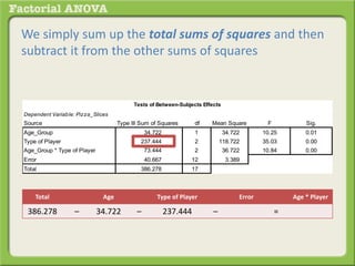
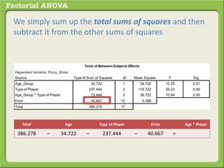
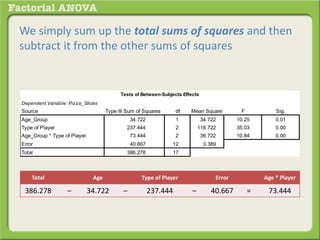
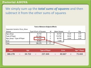
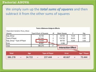
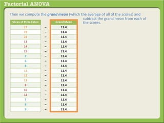
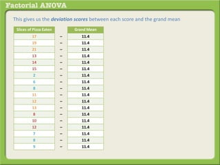
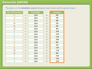
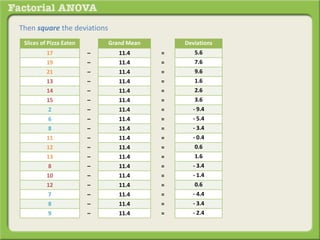
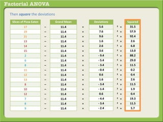
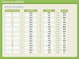
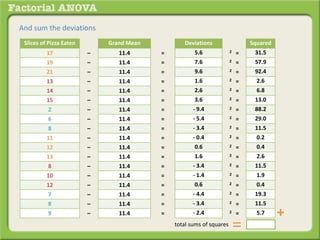
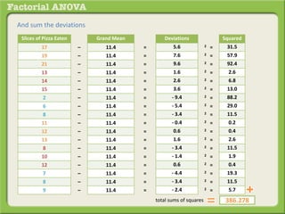
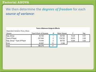
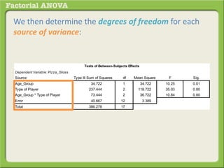
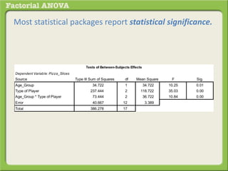
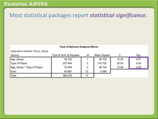
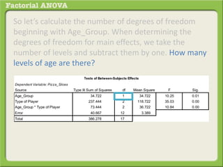
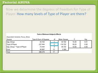
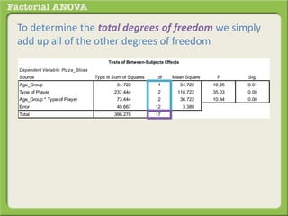
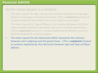
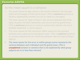
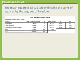
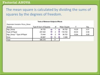
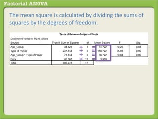
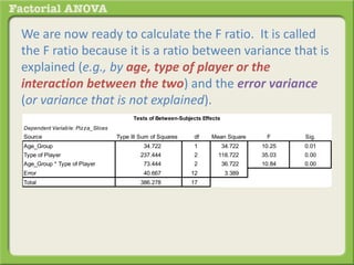
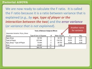
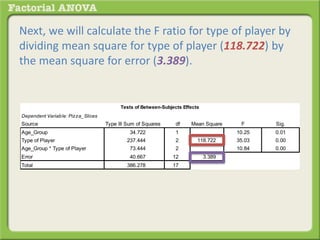
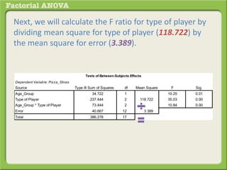
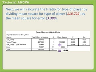
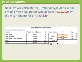
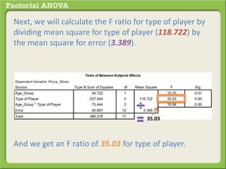
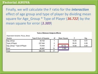
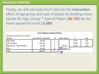
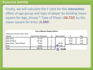
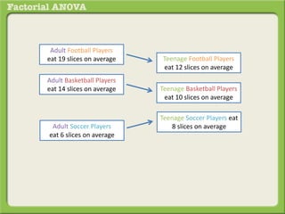
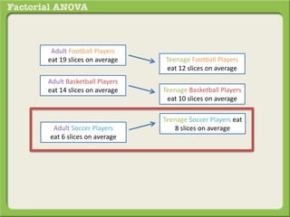
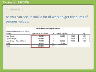
Factorial ANOVA

Factorial Analysis of Variance

First we begin with a research question

Who eats more slices of pizza in one sitting:
football, basketball or soccer players. What
effect does age (comparing adults to teenagers)
have on the results?
First we begin with a research question

Who eats more slices of pizza in one sitting: football, basketball
or soccer players. What effect does age (comparing adults to
teenagers) have on the results?

Inferential DescriptiveIs this an / question?

Inferential DescriptiveIs this an / question?
It’s inferential because
the question does not
specify a specific group
of football, basketball, or
soccer players.

Inferential Descriptive
Is this a question?DifferenceRelationship Goodness of
Fit
Independence

Is this a DifferenceRelationship Goodness
of Fit
Independence question?

Is this a DifferenceRelationship Goodness
of Fit
Independence question?
It’s difference in terms of
amount of pizza
consumed across player
types and age.

Is this data set
DifferenceRelationship Goodness
of Fit
Independence
?Normal Skewed or Kurtotic

Is the data set
of Fit
Independence
?
Normal Skewed or Kurtotic
Ratio/IntervalOrdinalNominal

Are there
of Fit
Independence
?
1 Dependent Variable 2 or more Dependent Variables

Are there
of Fit
Independence
?
Amount of Pizza Slices
Consumed in one sitting

Are there
of Fit
Independence
1 Independent Variable 2 or more Independent Variables ?

Are there
of Fit
Independence
1 Independent Variable 2 or more Independent Variables ?
Player Type and Age

Are there
of Fit
Independence
1 Independent Variable 2 or more Independent Variables
?2 levels 3 or more levels

Are there
of Fit
Independence
?3 or more levels2 levels

Are there
of Fit
Independence
?3 or more levels
3 levels for player type: football, basketball, soccer
2 levels for Age: teenager / adult
2 levels

of Fit
Independence
2 levels 3 or more levels
Are the samples ?Independent Repeated

of Fit
Independence
Are the samples ?Independent Repeated
The same individuals are not being measured repeatedly
and therefore are independent

of Fit
Independence
Independent Repeated
Will covariates no covariates be analyzed?

of Fit
Independence
Will covariates no covariates be analyzed?
For example, we will not be analyzing the difference
between athletes after eliminating the influence of age
(that would have made age a covariate)

of Fit
Independence
covariates no covariates
The appropriate analytical method based our answers to these questions is . . .

of Fit
Independence
covariates no covariates
The appropriate analytical method based our answers to these questions is . . .
Factorial
ANOVA

Thus far we have only considered one dependent
variable and one independent variable that was
categorized into several levels
One dependent variable
Dependent Variable: Amount of pizza eaten

One independent variable

Independent Variable: Athletes

Categorized into several levels

Level 1:
Football Player

Level 1:
Football Player
Level 2:
Basketball Player

Level 1:
Football Player
Level 2:
Basketball Player
Level 3:
Soccer Player

We can consider the effect of multiple independent
variables on a single dependent variable.

For example:

For example:
First Independent Variable: Athletes
Level 1:
Football Player
Level 2:
Basketball Player
Level 3:
Soccer Player

For example:
Level 1:
Football Player
Level 2:
Basketball Player
Level 3:
Soccer Player
Second Independent Variable: Age

For example:
Level 1:
Football Player
Level 2:
Basketball Player
Level 3:
Soccer Player
Second Independent Variable: Age
Level 1:
Adults
Level 2:
Teenagers

For example: the differences in number of slices of
pizza consumed (this is the single independent variable)
among 3 different athlete groups (Football, Basketball,
& Soccer) at two different age levels (Adults &
Teenagers).

Teenagers). Now, rather than comparing only 3 groups,
we will be comparing 6 groups (3 levels of athlete x 2
levels of age groups).

Teenagers). Now, rather than comparing only 3 groups,
we will be comparing 6 groups (3 levels of athlete x 2
levels of age groups).
Let’s see what this data set might look like.

First we list our three levels of athletes

First we list our three levels of athletes
Athletes
Football Player 1
Football Player 2
Football Player 3
Football Player 4
Football Player 5
Football Player 6
Basketball Player 1
Basketball Player 2
Basketball Player 3
Basketball Player 4
Basketball Player 5
Basketball Player 6
Soccer Player 1
Soccer Player 2
Soccer Player 3
Soccer Player 4
Soccer Player 5
Soccer Player 6

Then our two age groups
Athletes
Football Player 1
Football Player 2
Football Player 3
Football Player 4
Football Player 5
Football Player 6
Basketball Player 1
Basketball Player 2
Basketball Player 3
Basketball Player 4
Basketball Player 5
Basketball Player 6
Soccer Player 1
Soccer Player 2
Soccer Player 3
Soccer Player 4
Soccer Player 5
Soccer Player 6

Then our two age groups
Athletes Adults Teenagers
Football Player 1
Football Player 2
Football Player 3
Football Player 4
Football Player 5
Football Player 6
Basketball Player 1
Basketball Player 2
Basketball Player 3
Basketball Player 4
Basketball Player 5
Basketball Player 6
Soccer Player 1
Soccer Player 2
Soccer Player 3
Soccer Player 4
Soccer Player 5
Soccer Player 6

Now we add our dependent variable - pizza consumed
Football Player 1
Football Player 2
Football Player 3
Football Player 4
Football Player 5
Football Player 6
Basketball Player 1
Basketball Player 2
Basketball Player 3
Basketball Player 4
Basketball Player 5
Basketball Player 6
Soccer Player 1
Soccer Player 2
Soccer Player 3
Soccer Player 4
Soccer Player 5
Soccer Player 6

Now we add our dependent variable - pizza consumed
Football Player 1 9
Football Player 2 10
Basketball Player 1 1
Soccer Player 1 1
Soccer Player 2 2
Soccer Player 3 3
Soccer Player 4 2
Soccer Player 5 3
Soccer Player 6 5

The procedure by which we analyze the sums of
squares among the 6 groups based on 2 independent
variables (Age Group and Athlete Category) is called
Factorial ANOVA.

The procedure by which we analyze the sums of
squares among the 6 groups based on 2 independent
variables (Age Group and Athlete Category) is called
Factorial ANOVA.
sums of squares
between groups
sums of squares
within groups
degrees of freedom
means square
F ratio & F critical
hypothesis testing
one-way
ANOVA
factorial
ANOVA

Factorial ANOVA partitions the total sums of squares
into the unexplained variable and the variance
explained by the main effects of each of the
independent variables and the interaction of the
independent variables.

Factorial ANOVA partitions the total sums of squares
into the unexplained variable and the variance
explained by the main effects of each of the
independent variables and the interaction of the
independent variables.
Main Effect Interaction Effect Error
Explained Variance Type of Athlete
Age group
Type of Athlete by
Age Group
Unexplained Variance Within Groups

Continuing our example:
• The type of athlete may have an effect on the
number of slices of pizza eaten.

• But also the age group might as well have an effect
on the number of slices eaten.

• And the interaction of type of athlete and age group
may have an effect on slices eaten as well

• And the interaction of type of athlete and age group
may have an effect on slices eaten as well
In other words, some age groups within different athlete
categories may consume different amounts of pizza. For
example, maybe football and basketball adults eat much
more than football and basketball teenagers, while adult
soccer players eat much less than teenage soccer players.

In that case, the soccer players did not follow the trend
of the football and basketball players. This would be
considered an interaction effect between age group
and type of athlete.

Of course, there are 6 (3 x 2) possible combinations of
age groups and types of athletes any one of which may
not follow the direct main effect trend of age group or
type of athlete.

Of course, there are 6 (3 x 2) possible combinations of
age groups and types of athletes any one of which may
not follow the direct main effect trend of age group or
type of athlete.
• Adult Football Player
• Teenage Football Player
• Adult Basketball Player
• Teenage Basketball Player
• Adult Soccer Player
• Teenage Soccer Player

You could also order them this way:

The order doesn’t really matter.

When subgroups respond differently under different
conditions, we say that an interaction has occurred.

Adult Football Players
eat 19 slices on average Teenage Football Players
eat 12 slices on average

Adult Basketball Players
Teenage Football Players
Teenage Basketball Players

Do you see the trend here?

• Football players consume more pizza slices in one sitting
than do basketball players

• And adults consume more pizza slices than do teenagers

Now let’s add the soccer players

Now let’s add the soccer players
Adult Soccer Players
Teenage Soccer Players eat
8 slices on average

Because the soccer players do not follow the trend of
the other two groups, this is called an interaction effect
between type of athlete and age group.

So in the case below there would be no interaction
effect because all of the trends are the same:

eat 8 slices on average Teenage Soccer Players eat
6 slices on average

• As you get older you eat more slices of pizza
• If you play football you eat more than basketball and
soccer players
• etc.
6 slices on average

But in our first case there is an interaction effect
because one of the subgroups is not following the
trend:

trend:
8 slices on average

trend:
• Soccer players do not follow the trend of the older you
are the more pizza you eat.
8 slices on average

A factorial ANOVA will have at the very least three null
hypotheses. In the simplest case of two independent
variables, there will be three.

Here they are:

Here they are:
• Main Effect for Age Group: There is no significant
difference between the amount of pizza slices eaten by
adults and teenagers in one sitting.

Here they are:
• Main Effect for Type of Athlete: There is no significant
football, basketball, and soccer players in one sitting.

Here they are:
• Main Effect for Type of Athlete: There is no significant
• Interaction Effect Between Age Group and Type of
Athlete: There is no significant interaction between the
amount of pizza eaten by football, basketball and soccer
players in one sitting.

Let’s begin with the main effect for Age Group

Adults
eat 13 slices on average Teenagers

So adults eat 3 slices on average more than teenagers.
Is this a statistically significant difference? That’s what
we will find out using sums of squares logic.
Adults
eat 13 slices on average Teenagers

Now let’s look at main effect for Type of Athlete

Football Players
eat 15.5 slices on average
Basketball Players
Soccer Players
eat 7slices on average

So Football Players eat on average 5.5 slices more than
Basketball Players; Basketball Players eat 3 more slices
on average than Soccer Players; and Football Players
eat 8.5 slices on average more than Soccer Players.
Football Players
Basketball Players
Soccer Players

So Football Players eat on average 5.5 slices more than
Basketball Players; Basketball Players eat 3 more slices
on average than Soccer Players; and Football Players
eat 8.5 slices on average more than Soccer Players. Is
this a statistically significant difference? That’s what we
will find out using sums of squares logic.
Football Players
Basketball Players
Soccer Players

Finally let’s consider the interaction effect

8 slices on average

As noted in this example earlier, it appears that there
will be an interaction effect between Age Group and
Types of Athletes.
8 slices on average

So how do we test these possibilities statistically?

Factorial ANOVA will produce an F-ratio for each main
effect and for each interaction.

• Main effect: Age Group

• Main effect: Age Group – F ratio.

• Main effect: Type of Athlete

• Main effect: Type of Athlete – F ratio.

• Interaction effect: Age Group by Type of Athlete

• Interaction effect: Age Group by Type of Athlete – F ratio

• Interaction effect: Age Group by Type of Athlete – F ratio
Each of these F ratios will be compared with their
individual F-critical values on the F distribution table to
determine if the null hypothesis will be retained or
rejected.

Always interpret the F-ratio for the interactions effect
first, before considering the F-ratio for the main effects.

8 slices on average

If the F-ratio for the interaction is significant, the results
for the main effects may be moot.
8 slices on average

If the interaction is significant, it is extremely helpful to
plot the interaction to determine where the effect is
occurring.

If the interaction is significant, it is extremely helpful to
plot the interaction to determine where the effect is
occurring.
Notice how you can tell
visually that soccer players
are not following the age
trend as is the case with
football and basketball
players.

This looks a lot like our earlier image:

This looks a lot like our earlier image:
8 slices on average

There are many possible combinations of effects that
can render a significant F-ratio for the interaction. In
our example, one of the 6 groups might respond very
differently than the others …

There are many possible combinations of effects that
can render a significant F-ratio for the interaction. In
our example, one of the 6 groups might respond very
differently than the others … or 2, or 3, or … it can be
very complex.

If the interaction is significant, it is the primary focus of
interpretation.

interpretation.
However, sometimes the main effects may be
significant and meaningful; even the presence of the
significant interaction. The plot will help you decide if it
is meaningful.

interpretation.
However, sometimes the main effects may be
significant and meaningful; even the presence of the
significant interaction. The plot will help you decide if it
is meaningful.
For example, if all players increase in pizza consumption
as they age but some increase much faster in than
others, both the interaction and the main effect for age
may be important.

If the interaction is not significant, it can be ignored and
the interpretation of the main effects is
straightforward,

straightforward, as would be the case in this example:

straightforward, as would be the case in this example:
6 slices on average

You will now see how to calculate a Factorial ANOVA by
hand. Normally you will use a statistical software
package to do this calculation. That being said, it is
important to see what is going on behind the scenes.

Here is the data set we will be working with:

Here is the data set we will be working with:
Age Group Slices of Pizza Eaten Type of Player
Adult 17 Football Player
Adult 13 Basketball Player
Adult 2 Soccer Player
Teenage 11 Football Player
Teenage 8 Basketball Player
Teenage 7 Soccer Player

First we will compute the between group sums of squares for Age Group

Then we will compute the between group sums of squares for Type of Player

And then the sums of squares for the interaction effect

Then, we’ll round it off with the total sums of squares.

Once we have all of the sums of squares we can
produce an ANOVA table …

Dependent Variable: Pizza_Slices
Source Type III Sum of Squares df Mean Square F Sig.
Age_Group 34.722 1 34.722 10.25 0.01
Type of Player 237.444 2 118.722 35.03 0.00
Age_Group * Type of Player 73.444 2 36.722 10.84 0.00
Error 40.667 12 3.389
Total 386.278 17
Tests of Between-Subjects Effects

… that will make it possible to find the F-ratios we’ll
need to determine if we will reject or retain the null
hypothesis.
Age_Group 34.722 1 34.722 10.25 0.01
Type of Player 237.444 2 118.722 35.03 0.00
Error 40.667 12 3.389
Total 386.278 17

We begin with calculating Age Group Sums of Squares
Age_Group 34.722 1 34.722 10.25 0.01
Type of Player 237.444 2 118.722 35.03 0.00
Error 40.667 12 3.389
Total 386.278 17

We begin with calculating Age Group Sums of Squares
Here’s how we do it:
Age_Group 34.722 1 34.722 10.25 0.01
Type of Player 237.444 2 118.722 35.03 0.00
Error 40.667 12 3.389
Total 386.278 17

We organize the data set with Age Groups in the
headers,

headers,
Adults Teens
17 11
19 12
21 13
13 8
14 10
15 12
2 7
6 8
8 9

headers, then calculate the mean for each age group
Adults Teens
17 11
19 12
21 13
13 8
14 10
15 12
2 7
6 8
8 9

Adults Teens
17 11
19 12
21 13
13 8
14 10
15 12
2 7
6 8
8 9
mean

Adults Teens
17 11
19 12
21 13
13 8
14 10
15 12
2 7
6 8
8 9
mean 12.78

Adults Teens
17 11
19 12
21 13
13 8
14 10
15 12
2 7
6 8
8 9
mean 12.78 10.00

Then calculate the grand mean (which is the average of
all of the data)
Adults Teens
17 11
19 12
21 13
13 8
14 10
15 12
2 7
6 8
8 9
mean 12.78 10.00

all of the data)
Adults Teens
17 11
19 12
21 13
13 8
14 10
15 12
2 7
6 8
8 9
mean 12.78 10.00
grand mean

all of the data)
Adults Teens
17 11
19 12
21 13
13 8
14 10
15 12
2 7
6 8
8 9
mean 12.78 10.00
grand mean 11.39

all of the data)
Adults Teens
17 11
19 12
21 13
13 8
14 10
15 12
2 7
6 8
8 9
mean 12.78 10.00
grand mean 11.39 11.39

We subtract the grand mean from each age group
mean to get the deviation score
Adults Teens
17 11
19 12
21 13
13 8
14 10
15 12
2 7
6 8
8 9
mean 12.78 10.00

Adults Teens
17 11
19 12
21 13
13 8
14 10
15 12
2 7
6 8
8 9
mean 12.78 10.00
dev.score

Adults Teens
17 11
19 12
21 13
13 8
14 10
15 12
2 7
6 8
8 9
mean 12.78 10.00
dev.score 1.39

Adults Teens
17 11
19 12
21 13
13 8
14 10
15 12
2 7
6 8
8 9
mean 12.78 10.00
dev.score 1.39 - 1.39

Then we square the deviations
Adults Teens
17 11
19 12
21 13
13 8
14 10
15 12
2 7
6 8
8 9
mean 12.78 10.00
dev.score 1.39 - 1.39

Adults Teens
17 11
19 12
21 13
13 8
14 10
15 12
2 7
6 8
8 9
mean 12.78 10.00
dev.score 1.39 - 1.39
sq.dev.

Adults Teens
17 11
19 12
21 13
13 8
14 10
15 12
2 7
6 8
8 9
mean 12.78 10.00
dev.score 1.39 - 1.39
sq.dev. 1.93

Adults Teens
17 11
19 12
21 13
13 8
14 10
15 12
2 7
6 8
8 9
mean 12.78 10.00
dev.score 1.39 - 1.39
sq.dev. 1.93 1.93

Then multiply each squared deviation by the number of persons (9). This is
called weighting the squared deviations. The more person, the heavier the
weighting, or larger the weighted squared deviation values.
Adults Teens
17 11
19 12
21 13
13 8
14 10
15 12
2 7
6 8
8 9
mean 12.78 10.00
dev.score 1.39 - 1.39
sq.dev. 1.93 1.93

Adults Teens
17 11
19 12
21 13
13 8
14 10
15 12
2 7
6 8
8 9
mean 12.78 10.00
dev.score 1.39 - 1.39
sq.dev. 1.93 1.93
wt. sq. dev.

Adults Teens
17 11
19 12
21 13
13 8
14 10
15 12
2 7
6 8
8 9
mean 12.78 10.00
dev.score 1.39 - 1.39
sq.dev. 1.93 1.93
wt. sq. dev. 17.36

Adults Teens
17 11
19 12
21 13
13 8
14 10
15 12
2 7
6 8
8 9
mean 12.78 10.00
dev.score 1.39 - 1.39
sq.dev. 1.93 1.93
wt. sq. dev. 17.36 17.36

Finally, sum up the weighted squared deviations to get
the sums of squares for age group.
Adults Teens
17 11
19 12
21 13
13 8
14 10
15 12
2 7
6 8
8 9
mean 12.78 10.00
dev.score 1.39 - 1.39
sq.dev. 1.93 1.93
wt. sq. dev. 17.36 17.36

Finally, sum up the weighted squared deviations to get
the sums of squares for age group.
Adults Teens
17 11
19 12
21 13
13 8
14 10
15 12
2 7
6 8
8 9
mean 12.78 10.00
dev.score 1.39 - 1.39
sq.dev. 1.93 1.93
wt. sq. dev. 17.36 17.36 34.722

Note – this is the value from the ANOVA Table shown
previously:

Note – this is the value from the ANOVA Table shown
previously:
Age_Group 34.722 1 34.722 10.25 0.01
Type of Player 237.444 2 118.722 35.03 0.00
Error 40.667 12 3.389
Total 386.278 17

Next we calculate the Type of Player Sums of Squares

Next we calculate the Type of Player Sums of Squares
Age_Group 34.722 1 34.722 10.25 0.01
Type of Player 237.444 2 118.722 35.03 0.00
Error 40.667 12 3.389
Total 386.278 17

We reorder the data so that we can calculate sums of
squares for Type of Player

We reorder the data so that we can calculate sums of
squares for Type of Player
Football Basketball Soccer
17 13 2
19 14 6
21 15 8
11 8 7
12 10 8
13 12 9

Calculate the mean for each Type of Player
17 13 2
19 14 6
21 15 8
11 8 7
12 10 8
13 12 9

Calculate the mean for each Type of Player
17 13 2
19 14 6
21 15 8
11 8 7
12 10 8
13 12 9
mean 15.50 12.00 6.67

Calculate the grand mean (average of all of the scores)
17 13 2
19 14 6
21 15 8
11 8 7
12 10 8
13 12 9
mean 15.50 12.00 6.67

Calculate the grand mean (average of all of the scores)
17 13 2
19 14 6
21 15 8
11 8 7
12 10 8
13 12 9
mean 15.50 12.00 6.67
grand mean 11.4 11.4 11.4

Calculate the deviation between each group mean and
the grand mean(subtract grand mean from each
mean).
17 13 2
19 14 6
21 15 8
11 8 7
12 10 8
13 12 9
mean 15.50 12.00 6.67
grand mean 11.4 11.4 11.4

Calculate the deviation between each group mean and
the grand mean(subtract grand mean from each
mean).
17 13 2
19 14 6
21 15 8
11 8 7
12 10 8
13 12 9
mean 15.50 12.00 6.67
grand mean 11.4 11.4 11.4
dev.score 4.11 0.61 - 4.72

Square the deviations
17 13 2
19 14 6
21 15 8
11 8 7
12 10 8
13 12 9
mean 15.50 12.00 6.67
grand mean 11.4 11.4 11.4
dev.score 4.11 0.61 - 4.72

17 13 2
19 14 6
21 15 8
11 8 7
12 10 8
13 12 9
mean 15.50 12.00 6.67
grand mean 11.4 11.4 11.4
dev.score 4.11 0.61 - 4.72
sq.dev. 16.9 0.4 22.3

Weight the squared deviations
17 13 2
19 14 6
21 15 8
11 8 7
12 10 8
13 12 9
mean 15.50 12.00 6.67
grand mean 11.4 11.4 11.4
dev.score 4.11 0.61 - 4.72
sq.dev. 16.9 0.4 22.3

Weight the squared deviations
17 13 2
19 14 6
21 15 8
11 8 7
12 10 8
13 12 9
mean 15.50 12.00 6.67
grand mean 11.4 11.4 11.4
dev.score 4.11 0.61 - 4.72
sq.dev. 16.9 0.4 22.3
wt. sq. dev. 101.4 2.2 133.8

Sum the weighted squared deviations
17 13 2
19 14 6
21 15 8
11 8 7
12 10 8
13 12 9
mean 15.50 12.00 6.67
grand mean 11.4 11.4 11.4
dev.score 4.11 0.61 - 4.72
sq.dev. 16.9 0.4 22.3
wt. sq. dev. 101.4 2.2 133.8

Sum the weighted squared deviations
17 13 2
19 14 6
21 15 8
11 8 7
12 10 8
13 12 9
mean 15.50 12.00 6.67
grand mean 11.4 11.4 11.4
dev.score 4.11 0.61 - 4.72
sq.dev. 16.9 0.4 22.3
wt. sq. dev. 101.4 2.2 133.8 237.444

Here is the ANOVA table again:

Here is the ANOVA table again:
Age_Group 34.722 1 34.722 10.25 0.01
Type of Player 237.444 2 118.722 35.03 0.00
Error 40.667 12 3.389
Total 386.278 17

Here is how we reorder the data to calculate the within
groups sums of squares

Here is how we reorder the data to calculate the within groups sums of squares
Type of Player Age Group Slices of Pizza Eaten
Football Player Adult 17
Football Player Teenage 11
Basketball Player Adult 13
Basketball Player Teenage 8
Soccer Player Adult 2
Soccer Player Teenage 7

Calculate the mean for each subgroup
Type of Player Age Group Slices of Pizza Eaten

Calculate the mean for each subgroup
Type of Player Age Group Slices of Pizza Eaten Group Average
Football Player Adult 17 19
Football Player Teenage 11 12
Basketball Player Adult 13 14
Basketball Player Teenage 8 10
Soccer Player Adult 2 5
Soccer Player Teenage 7 8

Calculate the deviations by subtracting the group average from each athlete’s pizza eaten:
Type of Player Age Group Slices of Pizza Eaten Group Average

Calculate the deviations by subtracting the group average from each athlete’s pizza eaten:
Type of Player Age Group Slices of Pizza Eaten Group Average Deviations
Football Player Adult 17 19 - 2.0
Football Player Adult 19 19 0
Football Player Adult 21 19 2.0
Football Player Teenage 11 12 - 1.0
Football Player Teenage 12 12 0
Football Player Teenage 13 12 1.0
Basketball Player Adult 13 14 - 1.0
Basketball Player Adult 14 14 0
Basketball Player Adult 15 14 1.0
Basketball Player Teenage 8 10 - 2.0
Basketball Player Teenage 10 10 0
Basketball Player Teenage 12 10 2.0
Soccer Player Adult 2 5 - 3.3
Soccer Player Adult 6 5 0.7
Soccer Player Teenage 7 8 - 1.0
Soccer Player Teenage 8 8 0
Soccer Player Teenage 9 8 1.0

Type of Player Age Group Slices of Pizza Eaten Group Average Deviations
Football Player Adult 17 19 - 2.0
Football Player Adult 19 19 0
Football Player Adult 21 19 2.0
Football Player Teenage 11 12 - 1.0
Football Player Teenage 12 12 0
Football Player Teenage 13 12 1.0
Basketball Player Adult 13 14 - 1.0
Basketball Player Adult 14 14 0
Basketball Player Adult 15 14 1.0
Basketball Player Teenage 8 10 - 2.0
Basketball Player Teenage 10 10 0
Basketball Player Teenage 12 10 2.0
Soccer Player Adult 2 5 - 3.3
Soccer Player Teenage 7 8 - 1.0
Soccer Player Teenage 8 8 0
Soccer Player Teenage 9 8 1.0

Type of Player Age Group Slices of Pizza Eaten Group Average Deviations Squared
Football Player Adult 17 19 - 2.0 4.0
Football Player Adult 19 19 0 0
Football Player Adult 21 19 2.0 4.0
Football Player Teenage 11 12 - 1.0 1.0
Football Player Teenage 12 12 0 0
Football Player Teenage 13 12 1.0 1.0
Basketball Player Adult 13 14 - 1.0 1.0
Basketball Player Adult 14 14 0 0
Basketball Player Adult 15 14 1.0 1.0
Basketball Player Teenage 8 10 - 2.0 4.0
Basketball Player Teenage 10 10 0 0
Basketball Player Teenage 12 10 2.0 4.0
Soccer Player Adult 2 5 - 3.3 11.1
Soccer Player Adult 6 5 0.7 0.4
Soccer Player Teenage 7 8 - 1.0 1.0
Soccer Player Teenage 8 8 0 0
Soccer Player Teenage 9 8 1.0 1.0

Sum the squared deviations

sum of squares

40.7sum of squares

Age_Group 34.722 1 34.722 10.25 0.01
Type of Player 237.444 2 118.722 35.03 0.00
Error 40.667 12 3.389
Total 386.278 17

Here is a simple way we go about calculating sums of
squares for the interaction between type of athlete
and age group

Here is a simple way we go about calculating sums of
squares for the interaction between type of athlete
and age group
Age_Group 34.722 1 34.722 10.25 0.01
Type of Player 237.444 2 118.722 35.03 0.00
Error 40.667 12 3.389
Total 386.278 17

We simply sum up the total sums of squares and then
subtract it from the other sums of squares
Age_Group 34.722 1 34.722 10.25 0.01
Type of Player 237.444 2 118.722 35.03 0.00
Error 40.667 12 3.389
Total 386.278 17

Age_Group 34.722 1 34.722 10.25 0.01
Type of Player 237.444 2 118.722 35.03 0.00
Error 40.667 12 3.389
Total 386.278 17
Total Age Type of Player Error Age * Player
– – – =

Age_Group 34.722 1 34.722 10.25 0.01
Type of Player 237.444 2 118.722 35.03 0.00
Error 40.667 12 3.389
Total 386.278 17
386.278 – – – =

Age_Group 34.722 1 34.722 10.25 0.01
Type of Player 237.444 2 118.722 35.03 0.00
Error 40.667 12 3.389
Total 386.278 17
386.278 – 34.722 – – =

Age_Group 34.722 1 34.722 10.25 0.01
Type of Player 237.444 2 118.722 35.03 0.00
Error 40.667 12 3.389
Total 386.278 17
386.278 – 34.722 – 237.444 – =

Age_Group 34.722 1 34.722 10.25 0.01
Type of Player 237.444 2 118.722 35.03 0.00
Error 40.667 12 3.389
Total 386.278 17
386.278 – 34.722 – 237.444 – 40.667 =

Age_Group 34.722 1 34.722 10.25 0.01
Type of Player 237.444 2 118.722 35.03 0.00
Error 40.667 12 3.389
Total 386.278 17
386.278 – 34.722 – 237.444 – 40.667 = 73.444

Age_Group 34.722 1 34.722 10.25 0.01
Type of Player 237.444 2 118.722 35.03 0.00
Error 40.667 12 3.389
Total 386.278 17
386.278 – 34.722 – 237.444 – 40.667 = 73.444
Interaction Effect

So here is how we calculate sums of squares:

We line up our data in one column:
Slices of Pizza Eaten
17
19
21
13
14
15
2
6
8
11
12
13
8
10
12
7
8
9

Then we compute the grand mean (which the average of all of the scores) and
subtract the grand mean from each of
the scores.Slices of Pizza Eaten
17
19
21
13
14
15
2
6
8
11
12
13
8
10
12
7
8
9

Then we compute the grand mean (which the average of all of the scores) and
subtract the grand mean from each of
the scores.Slices of Pizza Eaten Grand Mean
17 – 11.4
19 – 11.4
21 – 11.4
13 – 11.4
14 – 11.4
15 – 11.4
2 – 11.4
6 – 11.4
8 – 11.4
11 – 11.4
12 – 11.4
13 – 11.4
8 – 11.4
10 – 11.4
12 – 11.4
7 – 11.4
8 – 11.4
9 – 11.4

This gives us the deviation scores between each score and the grand mean
Slices of Pizza Eaten Grand Mean
17 – 11.4
19 – 11.4
21 – 11.4
13 – 11.4
14 – 11.4
15 – 11.4
2 – 11.4
6 – 11.4
8 – 11.4
11 – 11.4
12 – 11.4
13 – 11.4
8 – 11.4
10 – 11.4
12 – 11.4
7 – 11.4
8 – 11.4
9 – 11.4

This gives us the deviation scores between each score and the grand mean
Slices of Pizza Eaten Grand Mean Deviations
17 – 11.4 = 5.6
19 – 11.4 = 7.6
21 – 11.4 = 9.6
13 – 11.4 = 1.6
14 – 11.4 = 2.6
15 – 11.4 = 3.6
2 – 11.4 = - 9.4
6 – 11.4 = - 5.4
8 – 11.4 = - 3.4
11 – 11.4 = - 0.4
12 – 11.4 = 0.6
13 – 11.4 = 1.6
8 – 11.4 = - 3.4
10 – 11.4 = - 1.4
12 – 11.4 = 0.6
7 – 11.4 = - 4.4
8 – 11.4 = - 3.4
9 – 11.4 = - 2.4

Then square the deviations
Slices of Pizza Eaten Grand Mean Deviations
17 – 11.4 = 5.6
19 – 11.4 = 7.6
21 – 11.4 = 9.6
13 – 11.4 = 1.6
14 – 11.4 = 2.6
15 – 11.4 = 3.6
2 – 11.4 = - 9.4
6 – 11.4 = - 5.4
8 – 11.4 = - 3.4
11 – 11.4 = - 0.4
12 – 11.4 = 0.6
13 – 11.4 = 1.6
8 – 11.4 = - 3.4
10 – 11.4 = - 1.4
12 – 11.4 = 0.6
7 – 11.4 = - 4.4
8 – 11.4 = - 3.4
9 – 11.4 = - 2.4

Then square the deviations
Slices of Pizza Eaten Grand Mean Deviations Squared
17 – 11.4 = 5.6 2 = 31.5
19 – 11.4 = 7.6 2 = 57.9
21 – 11.4 = 9.6 2 = 92.4
13 – 11.4 = 1.6 2 = 2.6
14 – 11.4 = 2.6 2 = 6.8
15 – 11.4 = 3.6 2 = 13.0
2 – 11.4 = - 9.4 2 = 88.2
6 – 11.4 = - 5.4 2 = 29.0
8 – 11.4 = - 3.4 2 = 11.5
11 – 11.4 = - 0.4 2 = 0.2
12 – 11.4 = 0.6 2 = 0.4
13 – 11.4 = 1.6 2 = 2.6
8 – 11.4 = - 3.4 2 = 11.5
10 – 11.4 = - 1.4 2 = 1.9
12 – 11.4 = 0.6 2 = 0.4
7 – 11.4 = - 4.4 2 = 19.3
8 – 11.4 = - 3.4 2 = 11.5
9 – 11.4 = - 2.4 2 = 5.7

And sum the deviations
17 – 11.4 = 5.6 2 = 31.5
19 – 11.4 = 7.6 2 = 57.9
21 – 11.4 = 9.6 2 = 92.4
13 – 11.4 = 1.6 2 = 2.6
14 – 11.4 = 2.6 2 = 6.8
15 – 11.4 = 3.6 2 = 13.0
2 – 11.4 = - 9.4 2 = 88.2
6 – 11.4 = - 5.4 2 = 29.0
8 – 11.4 = - 3.4 2 = 11.5
11 – 11.4 = - 0.4 2 = 0.2
12 – 11.4 = 0.6 2 = 0.4
13 – 11.4 = 1.6 2 = 2.6
8 – 11.4 = - 3.4 2 = 11.5
10 – 11.4 = - 1.4 2 = 1.9
12 – 11.4 = 0.6 2 = 0.4
7 – 11.4 = - 4.4 2 = 19.3
8 – 11.4 = - 3.4 2 = 11.5
9 – 11.4 = - 2.4 2 = 5.7

17 – 11.4 = 5.6 2 = 31.5
19 – 11.4 = 7.6 2 = 57.9
21 – 11.4 = 9.6 2 = 92.4
13 – 11.4 = 1.6 2 = 2.6
14 – 11.4 = 2.6 2 = 6.8
15 – 11.4 = 3.6 2 = 13.0
2 – 11.4 = - 9.4 2 = 88.2
6 – 11.4 = - 5.4 2 = 29.0
8 – 11.4 = - 3.4 2 = 11.5
11 – 11.4 = - 0.4 2 = 0.2
12 – 11.4 = 0.6 2 = 0.4
13 – 11.4 = 1.6 2 = 2.6
8 – 11.4 = - 3.4 2 = 11.5
10 – 11.4 = - 1.4 2 = 1.9
12 – 11.4 = 0.6 2 = 0.4
7 – 11.4 = - 4.4 2 = 19.3
8 – 11.4 = - 3.4 2 = 11.5
9 – 11.4 = - 2.4 2 = 5.7
total sums of squares

17 – 11.4 = 5.6 2 = 31.5
19 – 11.4 = 7.6 2 = 57.9
21 – 11.4 = 9.6 2 = 92.4
13 – 11.4 = 1.6 2 = 2.6
14 – 11.4 = 2.6 2 = 6.8
15 – 11.4 = 3.6 2 = 13.0
2 – 11.4 = - 9.4 2 = 88.2
6 – 11.4 = - 5.4 2 = 29.0
8 – 11.4 = - 3.4 2 = 11.5
11 – 11.4 = - 0.4 2 = 0.2
12 – 11.4 = 0.6 2 = 0.4
13 – 11.4 = 1.6 2 = 2.6
8 – 11.4 = - 3.4 2 = 11.5
10 – 11.4 = - 1.4 2 = 1.9
12 – 11.4 = 0.6 2 = 0.4
7 – 11.4 = - 4.4 2 = 19.3
8 – 11.4 = - 3.4 2 = 11.5
9 – 11.4 = - 2.4 2 = 5.7
386.278total sums of squares

And that’s how we calculate the total sums of squares
along with the interaction between Age Group and
Type of Player.

And that’s how we calculate the total sums of squares
along with the interaction between Age Group and
Type of Player.
Age_Group 34.722 1 34.722 10.25 0.01
Type of Player 237.444 2 118.722 35.03 0.00
Error 40.667 12 3.389
Total 386.278 17
386.278 – 34.722 – 237.444 – 40.667 = 73.444

We then determine the degrees of freedom for each
source of variance:
Age_Group 34.722 1 34.722 10.25 0.01
Type of Player 237.444 2 118.722 35.03 0.00
Error 40.667 12 3.389
Total 386.278 17

Why do we need to determine the degrees of
freedom?

freedom? Because this will make it possible to test our
three null hypotheses:

• Main effect for Age Group: There is NO significant difference
between the amount of pizza slices eaten by adults and
teenagers in one sitting.

• Main effect for Type of Player: There is NO significant

• Main effect for Type of Player: There is NO significant
• Interaction effect between Age Group and Type of Athlete:
There is NO significant interaction between the amount of
pizza slices eaten by football, basketball, and soccer players
in one sitting.

By dividing the sums of squares by the degrees of
freedom we can compute a mean square from which
we can compute an F ratio which can be compared to
the F critical.

the F critical.
Age_Group 34.722 1 34.722 10.25 0.01
Type of Player 237.444 2 118.722 35.03 0.00
Error 40.667 12 3.389
Total 386.278 17

the F critical.
If the F ratio is greater than the F critical, we would reject the null hypothesis
and determine that the result is statistically significant.
Age_Group 34.722 1 34.722 10.25 0.01
Type of Player 237.444 2 118.722 35.03 0.00
Error 40.667 12 3.389
Total 386.278 17

the F critical.
If the F ratio is greater than the F critical, we would reject the null hypothesis
and determine that the result is statistically significant. If the F ratio is smaller
than the F critical then we would fail to reject the null hypothesis.
Age_Group 34.722 1 34.722 10.25 0.01
Type of Player 237.444 2 118.722 35.03 0.00
Error 40.667 12 3.389
Total 386.278 17

Most statistical packages report statistical significance.
Age_Group 34.722 1 34.722 10.25 0.01
Type of Player 237.444 2 118.722 35.03 0.00
Error 40.667 12 3.389
Total 386.278 17

Age_Group 34.722 1 34.722 10.25 0.01
Type of Player 237.444 2 118.722 35.03 0.00
Error 40.667 12 3.389
Total 386.278 17
This means that if we
took 1000 samples we
would be wrong 1 time.
We just don’t know if
this is that time.

But it is important to know where this value came
from.
Age_Group 34.722 1 34.722 10.25 0.01
Type of Player 237.444 2 118.722 35.03 0.00
Error 40.667 12 3.389
Total 386.278 17
This means that if we
took 1000 samples we
would be wrong 1 time.
We just don’t know if
this is that time.

So let’s calculate the number of degrees of freedom
beginning with Age_Group.

beginning with Age_Group. When determining the
degrees of freedom for main effects, we take the
number of levels and subtract them by one.

number of levels and subtract them by one. How many
levels of age are there?

Adults Teens
17 11
19 12
21 13
13 8
14 10
15 12
2 7
6 8
8 9

Adults Teens
17 11
19 12
21 13
13 8
14 10
15 12
2 7
6 8
8 9
2 – 1 = 1 degree of freedom for age

Age_Group 34.722 1 34.722 10.25 0.01
Type of Player 237.444 2 118.722 35.03 0.00
Error 40.667 12 3.389
Total 386.278 17

Now we determine the degrees of freedom for Type of
Player.

Player. How many levels of Type of Player are there?

17 13 2
19 14 6
21 15 8
11 8 7
12 10 8
13 12 9

17 13 2
19 14 6
21 15 8
11 8 7
12 10 8
13 12 9
3 – 1 = 2 degrees of freedom for
type of player

Age_Group 34.722 1 34.722 10.25 0.01
Type of Player 237.444 2 118.722 35.03 0.00
Error 40.667 12 3.389
Total 386.278 17

To determine the degrees of freedom for the
interaction effect between age and type of player you
multiply the degrees of freedom for age by the degrees
of freedom for type of player.

1 * 2 = 2 degrees of freedom for
interaction effect

Age_Group 34.722 1 34.722 10.25 0.01
Type of Player 237.444 2 118.722 35.03 0.00
Error 40.667 12 3.389
Total 386.278 17

We now determine the degrees of freedom for error.

Here we take the number of subjects (18) and subtract
that number by the number of subgroups (6):

18 – 6 = 12 degrees of freedom for error

Age_Group 34.722 1 34.722 10.25 0.01
Type of Player 237.444 2 118.722 35.03 0.00
Error 40.667 12 3.389
Total 386.278 17

To determine the total degrees of freedom we simply
add up all of the other degrees of freedom

To determine the total degrees of freedom we simply
add up all of the other degrees of freedom
Age_Group 34.722 1 34.722 10.25 0.01
Type of Player 237.444 2 118.722 35.03 0.00
Error 40.667 12 3.389
Total 386.278 17

We now calculate the mean square.

We now calculate the mean square. The reason this
value is called mean square because it represents the
average squared deviation of scores from the mean.

We now calculate the mean square. The reason this
value is called mean square because it represents the
average squared deviation of scores from the mean.
You will notice that this is actually the definition for
variance.

So the mean square is a variance.

• The mean square for Age_Group is the variance between the two ages
(adult and teenager) and the grand mean. (This is explained variance or
variance explained by whether you are an adult or a teenager)

• The mean square for Type of Player is the variance between the three
types of player (football, basketball, and soccer) and the grand mean.
(This is explained variance or variance explained by whether you are a
football, basketball, or soccer player)

• The mean square for the interaction effect represents the variance
between each subgroup and the grand mean. (This is explained variance
or variance explained by the interaction between Age and Type of Player
effects)

• The mean square for the interaction effect represents the variance
between each subgroup and the grand mean. (This is explained variance
or variance explained by the interaction between Age and Type of Player
effects)
• The mean square for the error or within groups scores represents the
variance between each individual and the grand mean. (This is
unexplained variance or variance that is not explained by what group
subjects are in or how they interact)

The mean square is calculated by dividing the sums of
squares by the degrees of freedom.

The mean square is calculated by dividing the sums of
squares by the degrees of freedom.
Age_Group 34.722 1 34.722 10.25 0.01
Type of Player 237.444 2 118.722 35.03 0.00
Error 40.667 12 3.389
Total 386.278 17

We are now ready to calculate the F ratio. It is called
the F ratio because it is a ratio between variance that is
explained (e.g., by age, type of player or the
interaction between the two) and the error variance
(or variance that is not explained).

Age_Group 34.722 1 34.722 10.25 0.01
Type of Player 237.444 2 118.722 35.03 0.00
Error 40.667 12 3.389
Total 386.278 17

Age_Group 34.722 1 34.722 10.25 0.01
Type of Player 237.444 2 118.722 35.03 0.00
Error 40.667 12 3.389
Total 386.278 17
Another name
for variance

First we will calculate the F ratio for Age_Group by
dividing mean square for Age_Group (34.722) by the
mean square for error (3.389)

Age_Group 34.722 1 34.722 10.25 0.01
Type of Player 237.444 2 118.722 35.03 0.00
Error 40.667 12 3.389
Total 386.278 17

Age_Group 34.722 1 34.722 10.25 0.01
Type of Player 237.444 2 118.722 35.03 0.00
Error 40.667 12 3.389
Total 386.278 17
10.25

And we get an F ratio of 10.25 for Age_Group
Age_Group 34.722 1 34.722 10.25 0.01
Type of Player 237.444 2 118.722 35.03 0.00
Error 40.667 12 3.389
Total 386.278 17
10.25

The significance value of 0.01 means that if we were to
take 100 samples with the same Factorial Design and
analyze the results we would be wrong to reject the
null hypothesis 1 time.

The significance value of 0.01 means that if we were to
take 100 samples with the same Factorial Design and
analyze the results we would be wrong to reject the
null hypothesis 1 time. Because we are probably
comfortable with those odds, we will reject the null
hypothesis that age group has no effect on pizza
consumption.

Next, we will calculate the F ratio for type of player by
dividing mean square for type of player (118.722) by
the mean square for error (3.389).

Age_Group 34.722 1 34.722 10.25 0.01
Type of Player 237.444 2 118.722 35.03 0.00
Error 40.667 12 3.389
Total 386.278 17

Age_Group 34.722 1 34.722 10.25 0.01
Type of Player 237.444 2 118.722 35.03 0.00
Error 40.667 12 3.389
Total 386.278 17
35.03

And we get an F ratio of 35.03 for type of player.
Age_Group 34.722 1 34.722 10.25 0.01
Type of Player 237.444 2 118.722 35.03 0.00
Error 40.667 12 3.389
Total 386.278 17
35.03

The significance value of 0.00 (which, let’s say, is 0.002)
means that if we were to take 1000 samples with the
same factorial design and analyze the results we would
be wrong to reject the null hypothesis 2 times.

The significance value of 0.00 (which, let’s say, is 0.002)
be wrong to reject the null hypothesis 2 times. Because
we are probably comfortable with those odds, we will
reject the null hypothesis that type of player has no
effect on pizza consumption.

Finally, we will calculate the F ratio for the interaction
effect of age group and type of player by dividing mean
square for Age_Group * Type of Player (36.722) by the

Age_Group 34.722 1 34.722 10.25 0.01
Type of Player 237.444 2 118.722 35.03 0.00
Error 40.667 12 3.389
Total 386.278 17

Age_Group 34.722 1 34.722 10.25 0.01
Type of Player 237.444 2 118.722 35.03 0.00
Error 40.667 12 3.389
Total 386.278 17
10.84

And we get an F ratio of 10.84 for Age_Group * Type of
Player
Age_Group 34.722 1 34.722 10.25 0.01
Type of Player 237.444 2 118.722 35.03 0.00
Error 40.667 12 3.389
Total 386.278 17
10.84

The significance value of 0.00 (which, let’s say, is .003)
be wrong to reject the null hypothesis 3 times.

reject the null hypothesis that Age_Group * Type of
Player has no interaction effect on pizza consumption.

reject the null hypothesis that Age_Group * Type of
Player has no interaction effect on pizza consumption.
Once again, this means that one of the subgroups is not
acting like one or more other subgroups.

means
8 slices on average

In summary:
As you can see, it took a lot of work to get the sums of
squares values.

In summary:
squares values.
Age_Group 34.722 1 34.722 10.25 0.01
Type of Player 237.444 2 118.722 35.03 0.00
Error 40.667 12 3.389
Total 386.278 17

In summary:
squares values.
But once we have the sums of squares values and the
degrees of freedom we use simple division to calculate
the mean square.
Age_Group 34.722 1 34.722 10.25 0.01
Type of Player 237.444 2 118.722 35.03 0.00
Error 40.667 12 3.389
Total 386.278 17

Factorial ANOVA

More Related Content

What's hot

Viewers also liked

Similar to Factorial ANOVA

More from Ken Plummer

Recently uploaded

Factorial ANOVA